Estimating hazard ratios
hazard.RmdOverview
This vignette describes the estimate_ipwhr function,
providing details of how hazard ratios are computed, the theoretical
background for the implementation, and some examples extending those
found in the causalRisk
manual. estimate_ipwhr and methods for its resulting
object hew as closely as possible to the API for
estimate_ipwrisk.
estimate_ipwhr fits a weighted Cox model with the
treatment variable as its only regressor, to estimate the causal effect
of the treatment on the outcome, presented as hazard ratios relative to
the reference group. In the case of a binary treatment, the procedure
maximizes the partial likelihood
\[ L(\beta) = \prod_{i{:} \Delta_{i} = 1} {% \left[\frac{\exp(\beta X_i)}{\Sigma_{j \in R(t_{i})} \hat{w}_{j} \exp(\beta X_j)}\right] }^{\hat{w}_{i}}, \]
where \(\Delta_{i}\) is an indicator of whether an event was observed before censoring for subject \(i\), \(X_i\) is the treatment indicator for subject \(i\), \(\beta\) is the regression coefficient corresponding to the log hazard ratio between the treatment groups, \(t_{i}\) is the time at which an event occurred for subject \(i\), \(R(t_{i})\) is the risk set at time \(t_{i}\), and \(\hat{w}_{i}\) is a weight for subject \(i\) [1] (note that a slight modification of the likelihood is needed in the presence of tied event times).
In models without missingness, weights are inverse probabilities of
treatment. When the model includes missingness, weights are the product
of inverse probabilities of treatment and missingness.
estimate_ipwhr does not currently support inverse
probability of censoring weights.
Model assumptions
The estimators of causal effects requires special assumptions. We focus on the core set of assumptions frequently used to support this class of semiparametric estimators: consistency, no inteference, no unmeasured confounders, positivity, no measurement error on exposures, confounders, or treatment, missing data are stratified missing completely at random, and all statistical models are correctly specified. Additonal details on these assumptions can be found in the causalRisk manual’s technical appendix.
In addition to those general assumptions, we make the proportional hazards assumption that the survival curves for the treatment groups have hazard functions that are proportional over time.
Since estimate_ipwhr does not currently support inverse
probability of censoring weights, we assume that censoring is
noninformative, that is the censoring hazard is independent of
survival time conditional on the treatment and being at risk.
Finally, estimate_ipwhr does not currently support
competing risks, so we assume there are no competing
risks.
Confidence intervals
The confidence intervals are computed using the robust standard
errors produced by the coxph function in the survival
package. For IP weighted linear and generalized linear models, the
robust standard errors have been shown to be conservative, having
coverage probabilities slightly greater than the nominal coverage [2]. The robust standard errors derived from a
weighted Cox PH model are also claimed to be conservative [3]. A recent simulation study found that a
bootstrap approach to confidence interval estimation resulted in
coverage probabilities close to the nominal level [4]. In the current version of the software, we
do not enable a bootstrap estimation of confidence intervals.
Basic usage
This example extends the section Summarizing
cumulative risk by treatment group from the causalRisk
manual, providing a hazard ratio for the treatment model instead of
cumulative risk curves.
As described in the aforementioned section, the model can be defined as follows.
models <- specify_models(identify_treatment(Statin),
                         identify_censoring(EndofEnrollment),
                         identify_outcome(Death))
But now, instead of calling estimate_ipwrisk to produce
cumulative risk estimates, we use estimate_ipwhr to
estimate hazard ratios. The object fit1_hr has class
hr.
fit1_hr <- estimate_ipwhr(example1,
                          models,
                          tau = 24,
                          labels = "Fit1")
The plot method is identical to the
forest_plot method, returning an object of class “ggplot”
giving the estimated hazard ratio and, by default, an \(0.05\) -level confidence interval.
Ratios relative to the reference group are provided for all treatment
groups. In this example, the treatment variable Statin has
only two levels: “Treat” and “Control”.
plot(fit1_hr) +
  ggtitle("Mortality hazard ratio in Example1 data")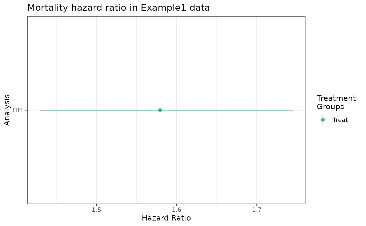
The make_table2 method when applied to
estimate_ipwhr objects behaves analogously to it’s
application to estimate_ipwrisk objects, producing
summaries on the hazard ratio scale rather than the risk difference or
relative ratio scales.
make_table2(fit1_hr)Both the plot and make_table2 methods allow
for specifying different confidence levels via the alpha
argument.
make_table2(fit1_hr, alpha = 0.01)Estimating hazard ratios with IPT weights
This example demonstrates the usage of estimate_ipwhr in
which an IPTW model is used to produce per-subject weights.
estimate_ipwhr fits the treatment model with
estimate_ipwrisk to the treatment weights, whose product is
passed a the weights argument to survival::coxph. See the
Overview section for a more technical description of that procedure.
models <- specify_models(identify_treatment(Statin, formula = ~DxRisk),
                         identify_censoring(EndofEnrollment),
                         identify_outcome(Death))
Here, we use the tau = 24 argument to specify the
maximum follow-up time during this study.
fit2_hr <- estimate_ipwhr(example1,
                          models,
                          tau = 24,
                          labels = "Fit2")
As with the cumrisk methods, hr class
plot and make_table2 methods support passing
multiple objects resulting from estimate_ipwhr. It is
important to provide unique labels to each object before passing them
into plot or make_table2.
plot(fit1_hr, fit2_hr) +
  ggtitle("Mortality hazard ratio in Example1 data")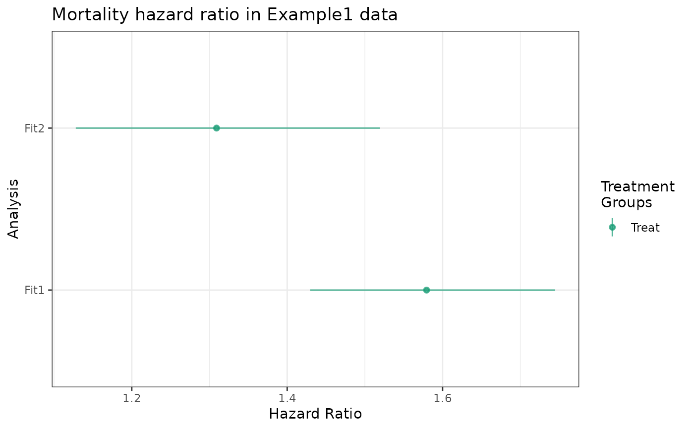
make_table2(fit1_hr, fit2_hr)Changing the reference group
The reference group for estimate_ipwhr can be changed
using the ref argument. Note that this is different
behavior from estimate_ipwrisk objects where the reference
group need not be specified until invoking the supporting methods such
as plot, make_table2, and
forest_plot. With estimate_ipwhr the reference
group can be set by providing a string specifying the name of the
desired reference level.
fit2_hr_treat <- estimate_ipwhr(example1,
                                models,
                                tau = 24,
                                labels = "Fit2, Treat is Ref",
                                ref = "Treat")

make_table2(fit2_hr, fit2_hr_treat)
Estimating hazard ratios with more than two treatment groups
estimate_ipwhr supports treatment variables with more
than two levels. This section extends Estimating
risk with more than two treatment groups from the causalRisk manual,
using analogous object names.
models <- specify_models(identify_treatment(StatinPotency, formula = ~DxRisk),
                         identify_censoring(EndofEnrollment),
                         identify_outcome(Death))

fit4_hr <- estimate_ipwhr(example1,
                          models,
                          tau = 24,
                          labels = "Fit4")
Ratios are relative to the “Control” group.
plot(fit4_hr) +
  ggtitle("Mortality hazard ratio in Example1 data")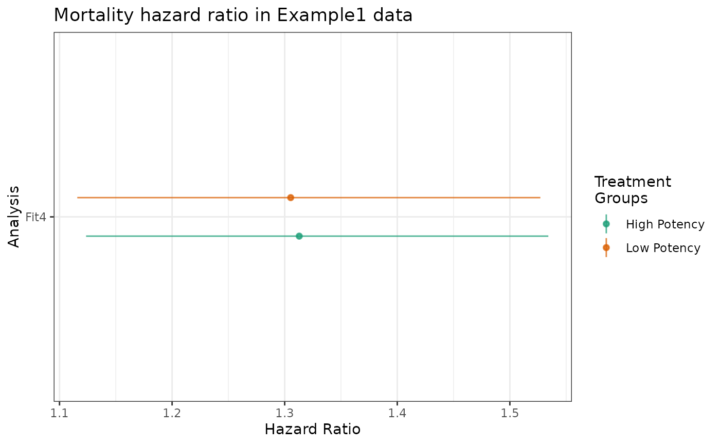
plot(fit1_hr, fit4_hr) +
  ggtitle("Mortality hazard ratio in Example1 data")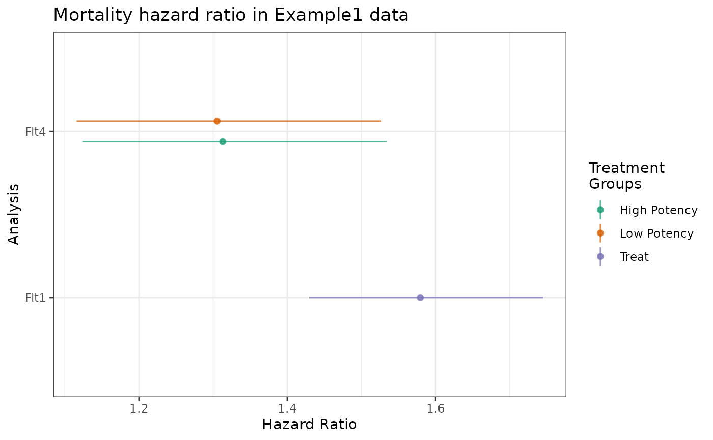
make_table2(fit1_hr, fit4_hr, alpha = 0.01)Extracting hr_data
The plot, forest_plot and
make_table2 methods for class hr rely on the
utility hr_data, which is exported for convenience. It
wraps the summary.coxph method, applying it to the
fitted_model field of the return object, and provides
counts of events and observations by treatment group.
The return value is a data frame, which row-binds the extracted fit
data for all hr fit objects provided.
For example, to retrieve a data frame with the data backing plot and table methods for the examples above,
hr_data(fit1_hr, fit2_hr, fit4_hr)## # A tibble: 7 × 7
## analysis n events group_label hr hr_lcl hr_ucl
## <chr> <int> <int> <chr> <dbl> <dbl> <dbl>
## 1 Fit1 6799 2099 Treat 1.58 1.43 1.74
## 2 Fit1 3201 470 Control NA NA NA
## 3 Fit2 6799 2099 Treat 1.31 1.13 1.52
## 4 Fit2 3201 470 Control NA NA NA
## 5 Fit4 3406 1053 High Potency 1.31 1.12 1.53
## 6 Fit4 3393 1046 Low Potency 1.31 1.12 1.53
## 7 Fit4 3201 470 Control NA NA NA