causalRisk manual

Overview

The causalRisk package aims to provide easy-to-use tools for estimating the cumulative risk of an outcome, including counterfactual outcomes, allowing for the estimation of causal effects. The estimators that are currently implemented within the package are types of inverse probability weighted estimators.[1] Currently, the package allows for the estimation of the cumulative risk of a right-censored counterfactual outcome, that may be subject to dependent (right) censoring, confounding, selection bias, and competing risks. The package also provides a range of helper functions to produce common plots and tables, and includes example data, vignettes, simulation functions, and testing and simulation scripts. The package also supports the estimation of counterfactual hazard ratios that may be subject to confounding and missingness.

The package also aims to create an R sub-language that will permit analyses to be expressed in a more human-readable form (as opposed to R programming statements). The sub-language will allow the user to describe a new analysis as a modification of an existing analysis, minimizing risk of errors from copying and pasting code and resulting in analysis statements that are more human readable. It is also hoped that the sub-language will be sufficiently general that it can be easily extended and modified to incorporate different estimation approaches as well as different estimands.

The manual is structured by way of examples.

Parallel processing

The package makes use of parallel processing via the future package.

library(causalRisk)
library(future)
plan("multisession")

Format of incoming data

The package expects incoming data to be supplied as an R data.frame. The package contains several example simulated data sets. The first simulated data set can be used to illustrate the use of causalRisk to solve a problem with censoring, a confounded treatment, and a competing event. The first twenty rows of the data example1 appear below:

example1[1:20, ] %>% kable

id	DxRisk	Frailty	Sex	Statin	StatinPotency	EndofEnrollment	Death	Discon	CvdDeath
1	0.933	-0.399	Male	Control	Control	2.316	NA	NA	NA
2	-0.525	-0.006	Female	Treat	Low Potency	0.210	NA	NA	NA
3	1.814	0.180	Male	Control	Control	6.629	NA	1.438	NA
4	0.083	0.388	Female	Treat	Low Potency	NA	34.2	16.215	1
5	0.396	-1.111	Male	Treat	High Potency	3.919	NA	NA	NA
6	-2.194	-1.030	Female	Treat	Low Potency	2.189	NA	0.102	NA
7	-0.360	0.582	Male	Control	Control	0.134	NA	NA	NA
8	0.143	1.263	Male	Control	Control	14.555	NA	0.165	NA
9	-0.204	-0.591	Male	Treat	Low Potency	NA	17.2	NA	0
10	0.446	-0.730	Female	Control	Control	0.400	NA	NA	NA
11	-0.322	1.317	Female	Treat	Low Potency	16.909	NA	6.065	NA
12	0.478	1.372	Female	Treat	High Potency	1.598	NA	NA	NA
13	0.196	-0.736	Male	Treat	Low Potency	0.106	NA	NA	NA
14	0.715	-0.212	Female	Control	Control	NA	15.5	NA	0
15	-0.960	-1.145	Male	Treat	High Potency	NA	5.4	2.781	0
16	0.671	-0.010	Male	Treat	High Potency	NA	22.3	NA	0
17	1.655	1.485	Female	Treat	Low Potency	20.458	NA	NA	NA
18	1.243	1.805	Female	Control	Control	22.903	NA	NA	NA
19	-1.562	-0.332	Female	Treat	High Potency	3.199	NA	0.170	NA
20	1.182	-0.764	Male	Control	Control	0.489	NA	NA	NA

The simulated data come from a hypothetical cohort study designed to look at the effectiveness of statin therapy in a routine care population with elevated lipids. We imagine that the data were generated from a treatment decision design[2], with the index date being the receipt of an elevated lipid test result in a treatment-naive patient. The variable Statin is a 2-level factor that indicates whether the patient was started on a statin agent after the receipt of the test result. The variable StatinPotency is a three-level factor that further indicates the potency of the statin agent (“high” versus “low”). The variable Death is the time of death in months after the start of treatment; CvdDeath is an indicator whether the patient died of cardiovascular disease; EndofEnrollment is the time in months until loss of health plan enrollment; and Discon is the time in months until treatment discontinuation. The time to event variable and the competing event indicator variable are missing if the event was not observed to have occurred. Several baseline variables (potential confounders, determinants of censoring) are also included in the data: Frailty, which is a summary measure of frailty; and DxRisk, which is a hypothetical measure of cardiovascular risk and a risk factor for the outcome. The simulated data also include the factor variable sex.

Note that the incoming data do not need to include indicators for censoring. These are created by the estimation functions in causalRisk. Variables that are censored should be set to NA. An event or censoring variable that is either NA or larger than the first observed event or censoring time is taken to be censored at the first observation of the outcome or other censoring variable.

Estimating the cumulative distribution of a right-censored outcome

For descriptive purposes, we are often interested in estimating the cumulative distribution of an outcome \(Y\), or \(F(t)=P(Y<t)\), in the overall population, subject to right-censoring by \(C\). Here we term this quantity the cumulative risk function. We can estimate it with the following inverse-probability of censoring weighted estimating function: \[ \hat{Pr}(Y<t)= \frac{1}{n}\sum_{i = 1}^{n} \frac{\Delta_i I(Y_i<t)}{\hat{Pr}(\Delta=1|T_i)}, \] where \(\Delta = I(Y<C)\) is an indicator that the patient was uncensored and \(T = min(Y, C)\) is the earlier of the event or censoring times.[3], [4] This estimating function depends on a single nuisance parameter: \(Pr(\Delta=1|T)\), the probability that an observation will be uncensored at the earlier of their observed censoring or event times. If the censoring probability is estimated with a Kaplan-Meier estimator then the resulting estimate of the cumulative risk is identical to the complement of the Kaplan-Meier estimate of the survival function of \(Y\).[5] The consistency of this estimator requires that censoring is non-informative or equivalently that \(C\) and \(Y\) are independent.[3]

Estimation and display of results

Prior to estimating the cumulative risk function, one must specify models and other features of the incoming data needed by the estimating procedures. This is accomplished using the function specify_models, which creates an object of class model_specification. The function takes as arguments descriptor functions to facilitate the construction of this object.

For the current estimation problem, we need to identify the outcome and the censoring variable. Here we identify the variable EndofEnrollment as a censoring variable and Death as the outcome variable:

models = specify_models(identify_censoring(EndofEnrollment),
                        identify_outcome(Death))

Given a model specification object identifying the censoring and outcome variables, we can now estimate the cumulative risk of the outcome using the function estimate_ipwrisk. The function takes other arguments (see help function and vignettes); below we specify the argument times, which identifies the time points at which estimate_ipwrisk estimates the cumulative risk; the label function simply assigns labels to the analysis which can be used to identify the analysis in plots and tables containing multiple analyses, as will be illustrated.

fit1 = estimate_ipwrisk(example1, models,
                   times = seq(0,24,0.1),
                   labels = c("Overall cumulative risk"))

The call to estimate_ipwrisk returns an object of type ipw for which various generic plot and table making methods are defined. For example, the generic function plot, will produce the cumulative incidence functions and confidence intervals:

plot(fit1)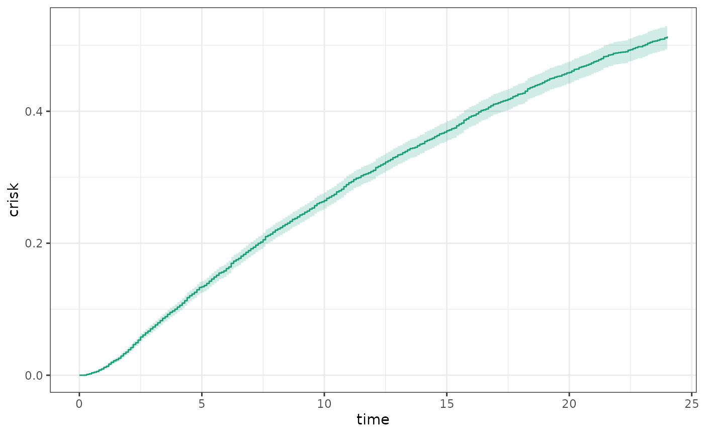

Plot returns a ggplot2 object and therefore can be modified using the extensive functionality of ggplot2, e.g.

plot(fit1) +  ylab("Cumulative risk") + 
  xlab("Time in months")

Estimating the cumulative risk of a right-censored outcome subject to dependent censoring

In many settings, it may be unrealistic to assume that censoring is non-informative. For example, if censoring occurs by loss of health plan enrollment and healthier patients are more likely to disenroll, then patients who remain under follow-up will tend to represent less healthy patients.

To the extent that the predictors of both disenrollment and the outcome of interest are accurately captured in the data, informative censoring can be addressed using the following inverse-probability of censored weighted estimator: \[ \hat{Pr}(Y<t)= \frac{1}{n}\sum_{i = 1}^{n} \frac{\Delta_i I(Y_i<t)}{\hat{Pr}(\Delta=1|W_i, T_i)}, \] where \(W\) is a set of baseline covariates, \(C\) is the time of censoring, \(\Delta = I(Y<C)\) is an indicator that the patient was uncensored, and \(T = min(Y, C)\) is the earlier of the event or censoring time. This estimating function depends on one nuisance parameter: \(Pr(\Delta=1|W, T)\), the conditional probability that an observation will be uncensored at the earlier of their observed event or censoring times given \(W\). It must be estimated according to an assumed model.

The consistency of this estimating function requires that \(C\) and \(Y\) are conditionally independent given \(W\) and that the model for \(Pr(\Delta=1|W_i, T_i)\) is correctly specified.[3],[4],[6]

Estimation

For the current estimation problem, we need to update the data structure object by identifying a model for the censoring variable. The default model is a Cox proportional hazards model, but it is necessary to specify which variables should be included in the model. This is done by specifying a formula. Here we request that the censoring model should contain the baseline variable DxRisk:

models_cens = specify_models(identify_censoring(EndofEnrollment, formula = ~DxRisk),
                      identify_outcome(Death))

fit1_cens = estimate_ipwrisk(example1, models_cens,
                     times = seq(0,24,0.1),
                     labels = c("Cumulative Risk of Mortality, IPCW"))

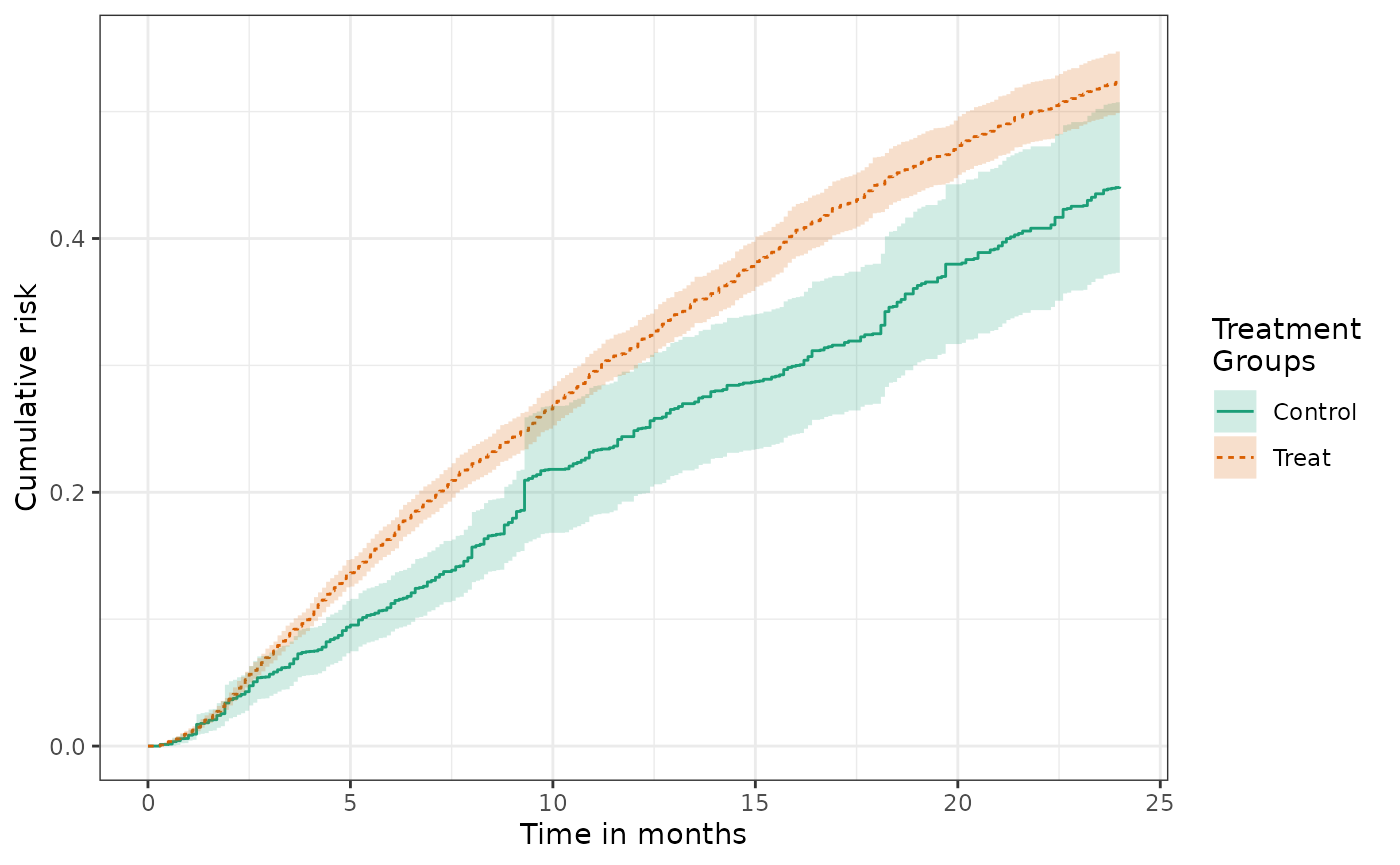
plot(fit1, fit1_cens, scales="fixed", overlay = TRUE)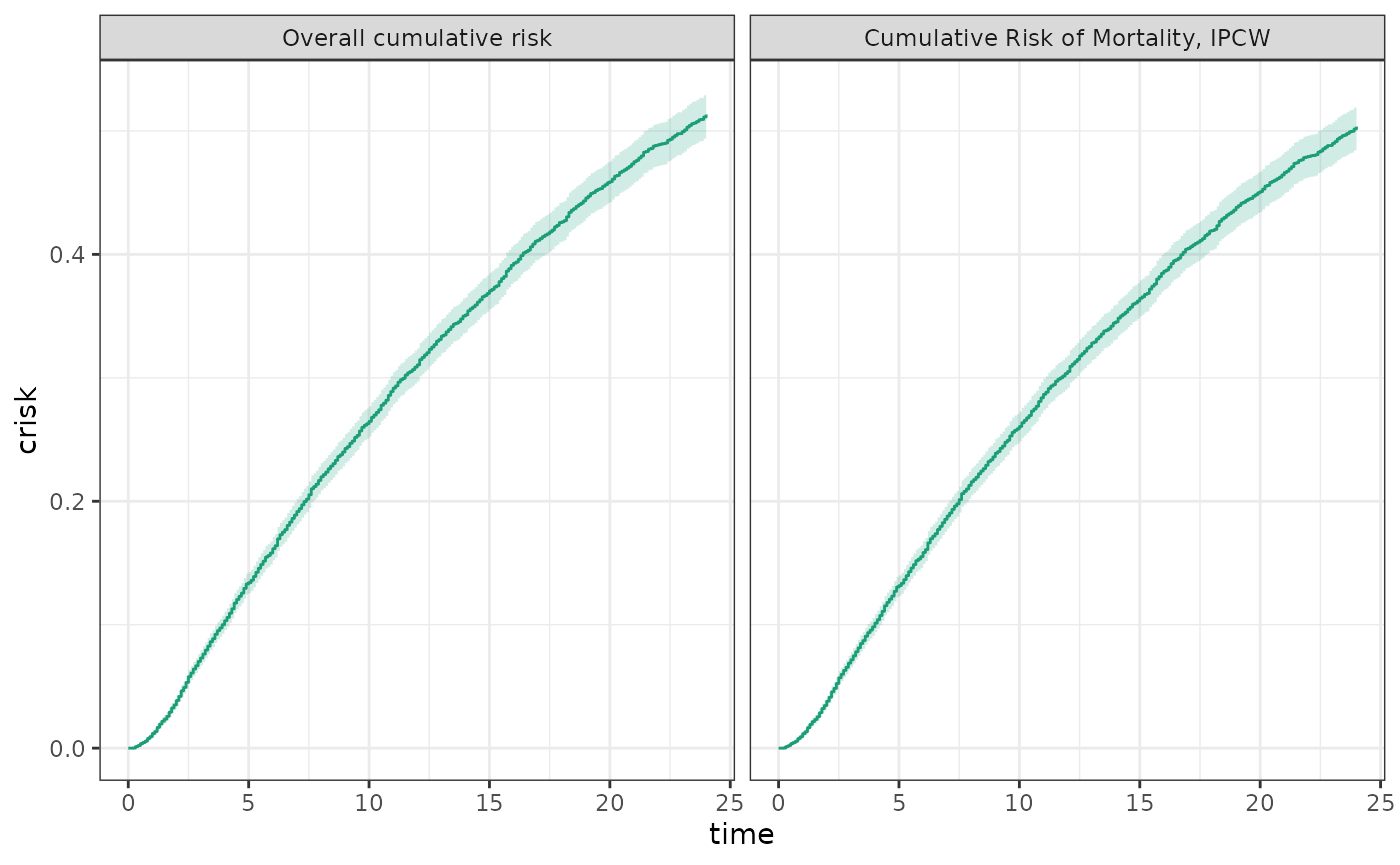

Competing risks

A competing risk is an event that precludes the occurrence of an event of interest.[7],[8] For example, death from cancer would be a competing risk for death from cardiovascular disease. In the competing risk formulation described here, the event time \(Y\) could either be the time of the competing event or the event of interest. We are interested in estimating the cumulative risk that the event of interest has occurred before the competing event by time \(t\), or \(F(t)=P(Y<t, J=1)\), where \(J\) is an indicator that \(Y\) is the time of the event of interest, rather than the competing event. \[ \hat{Pr}(Y<t, J=1) = \frac{1}{n}\sum_{i = 1}^{n} \frac{\Delta_{i} I(Y_i<t, J_{i}=1)}{\hat{Pr}(\Delta=1|W_i, T_i)}, \] As before this estimating function is allowing for the possibility of dependent censoring.

The consistency of this estimating function requires that \(C\) and \((Y, J)\) are conditionally independent given \(W\). We also require that the model for \(Pr(\Delta=1|W, T)\) is correctly specified.

Estimation

In the example data set, example1, the variable CvdDeath indicates whether Death is the event of interest or a competing event. To conduct a competing risks analysis, we can add a competing risk feature to the data structure object. This is done with the constructor function identify_competing_risk, which depends on parameters event and event_value. The parameter event contains the variable that identifies whether the outcome is the outcome of interest or a competing event; and event_value provides the value that the variable event takes when the event is the event of interest rather than a competing event. In the data structure, we identify CvdDeath as the event indicator variables and indicate that CvdDeath = 1 denotes the event of interest by specifying event_value = 1:

models_cr1 = specify_models(identify_censoring(EndofEnrollment, formula = ~DxRisk),
                      identify_competing_risk(name = CvdDeath, event_value = 1),
                      identify_outcome(Death))

As before the model can be fit using the function estimate_ipwrisk

fit1_cr1 = estimate_ipwrisk(example1, models_cr1, 
                   times=seq(0,24,0.1),
                   label=c("CV mortality, IPCW"))

In competing risks analysis, often one reports the cumulative incidence of the event of interest, as well as the cumulative incidence of the competing event and the composite of both the competing event and the event of interest.

models_cr0 = specify_models(identify_censoring(EndofEnrollment, formula = ~DxRisk),
                      identify_competing_risk(name = CvdDeath, event_value = 0),
                      identify_outcome(Death))


fit1_cr0 = estimate_ipwrisk(example1, models_cr0,
                     times = seq(0,24,0.1),
                     labels = c("Non-CV mortality, IPCW"))

plot(fit1_cens, fit1_cr1, fit1_cr0, ncol=3,
     scales="fixed", overlay = TRUE)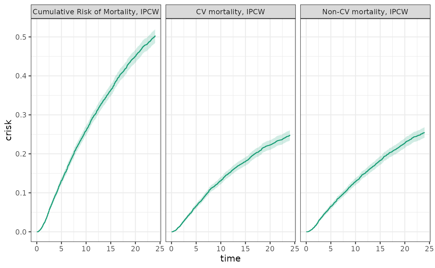

Also when the results are tabulated, the sum of the cumulative risks for each of the events should equal the composite risk. Basic statistics about events and risks at chosen time points can be generated using the table making function make_table2.

make_table2(fit1_cens, fit1_cr1, fit1_cr0)

Summarizing cumulative risk by treatment group

The cumulative risk can be computed by treatment groups. To do this, one needs to add the variable identifying the received treatment to the data structure object by using the constructor function identify_treatment:

models_treat = specify_models(identify_treatment(Statin),
                              identify_censoring(EndofEnrollment, formula = ~DxRisk),
                              identify_outcome(Death))

Now when estimate_ipwrisk is called, it returns a risk curve for each level of treatment:

fit1_treat = estimate_ipwrisk(example1, models_treat,
                   times = seq(0,24,0.1),
                   labels = c("Unadjusted cumulative risk"))

When this function is plotted one obtains an unadjusted cumulative risk for each treatment group.

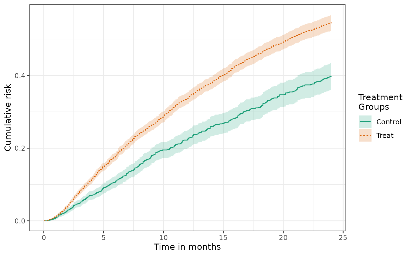
plot(fit1_treat) +ylab("Cumulative risk") + 
  xlab("Time in months")

Table 1: Summarizing patient characteristics by treatment group

In both randomized and non-experimental studies it is typical to report the means and frequencies of patient characteristics by treatment group. In randomized studies, this is done to ensure that the randomization achieves a good balance of patient risk factors across treatment arms. In non-experimental studies, this is done to understand the comparability of patient groups and to identify the presence and nature of possible confounding. The function make_table1 can be used to tabulate summary statistics of specified covariates by treatment group.

make_table1(example1, Statin, DxRisk, Frailty, Sex)

Characteristic¹	Control n=3201	Treat n=6799
DxRisk, Mean (SD)	0.74 (0.85)	-0.35 (0.88)
Frailty, Mean (SD)	0.01 (1.02)	0.02 (1.00)
Sex
Female	1581 49.39	3287 48.35
Male	1620 50.61	3512 51.65
¹ All values are N (%) unless otherwise specified

The functions takes as an argument a data.frame object, a factor variable identifying treatment groups, and the variables to be summarized supplied as additional arguments.

The functions can also present small histograms or density plots to graphically show the balance of characteristics across treatment groups.

make_table1(example1, Statin, DxRisk, Frailty, Sex, graph = TRUE)

Characteristic¹	Control n=3201	Treat n=6799
DxRisk, Mean (SD)	0.74 (0.85)	-0.35 (0.88)
Frailty, Mean (SD)	0.01 (1.02)	0.02 (1.00)
Sex
Female	1581 49.39	3287 48.35
Male	1620 50.61	3512 51.65
¹ All values are N (%) unless otherwise specified

Estimating the cumulative risk of a right-censored counterfactual outcome

To conduct causal inference about the effect of an assigned treatment, we are interested in estimating the cumulative distribution of treatment-specific counterfactual outcomes, \(F_a(t)=P(Y(a)<t)\). Here \(Y(a)\) is a (possibly) counterfactual outcome; the outcome that would have been observed if treatment were to have been assigned to \(a\), where \(a\) is drawn from a set of possible treatments, \(\mathcal{A}\).

To identify various causal effects, we must make a variety of additional assumptions including no unmeasured confounding, consistency, positivity, and no interference (see Assumptions needed for causal inference). Under these assumptions, we can estimate the cumulative distribution function \(Y(a)\) with the following estimating function: \[ \hat{Pr}(Y(a)<t)= \frac{1}{n}\sum_{i = 1}^{n} \frac{\Delta_i I(Y_i<t) I(A_i=a)}{Pr(\Delta=1|W_i,A_i, T_i) Pr(A=a|W_i)}, \] where \(A\) is the observed treatment.

This estimating function depends on two nuisance parameters: the censoring probability (as before), \(Pr(\Delta=1|W,A, T)\), and the propensity score (PS) or conditional probability of treatment given \(W\), \(Pr(A=a|W)\). These must be estimated according to assumed models. The current version of causalRisk defaults to a logistic model for \(Pr(A=a|W)\) and a Cox proportional hazards model for \(Pr(\Delta=1|W,A, T)\). Note that \(W\) represents a set of candidate covariates and the individual covariates included in the specific models need not be the same.

In addition to the assumptions required for causal inference, the consistency of this estimating function requires that \(C\) and \((Y(a), a \in \mathcal{A})\) are conditionally independent given \(W\) and that the model for \(Pr(\Delta=1|W, A, T)\) and \(Pr(A=a|W)\) are correctly specified.[4],[6]

Estimating counterfactual cumulative risk using causalRisk

To augment the model specification object to identify treatment groups and models, we use the constructor function identify_treatment:

models2 = specify_models(identify_treatment(Statin, formula = ~DxRisk ),
                         identify_censoring(EndofEnrollment, formula = ~DxRisk),
                         identify_outcome(Death))

This code identifies the variable Statin as the treatment, and specifies a model for its mean using a logistic regression model (the default) with a model formula ~DxRisk \[ Pr(A=1|W)=(1+exp(-\alpha W_1))^{-1} \] As before, the censoring variable is identified as EndofEnrollment with a model formula given by ~DxRisk. Note that because the censoring model conditions on treatment, the Cox model is estimated within each treatment group, thus there is no need to include the treatment variable in the model.

Given our data structure and assumed models for censoring and treatment, we can now estimate cumulative risk using the function estimate_ipwrisk:

fit2 = estimate_ipwrisk(example1, models2, 
                        times = seq(0,24,0.1),
                        labels = c("IPTW+IPCW main analysis"))

Note that the times argument here tells the functions at what times it should compute the cumulative incidence. The rate is computed through the end of follow-up or, if the times arguments provided, through the maximum of times. Alternatively, the argument tau can be used to set a maximum length of follow-up.

Plotting counterfactual cumulative risk and effect measures

The generic function plot, will produce the cumulative incidence functions for each treatment group and confidence intervals:

plot(fit2) + ylab("Cumulative risk") +
  xlab("Time in months")

The confidence intervals for the control group are wider because controls comprise only approximately 1/3 of the study population.

From these cumulative risk curves different causal contrasts can be constructed. Of central interest is often the cumulative risk difference: \[ RD(t) = P(Y(1) < t) - P(Y(0) < t). \]

The plot function can produce a plot of the estimated cumulative risk difference by setting the parameter effect_measure_type = "RD".

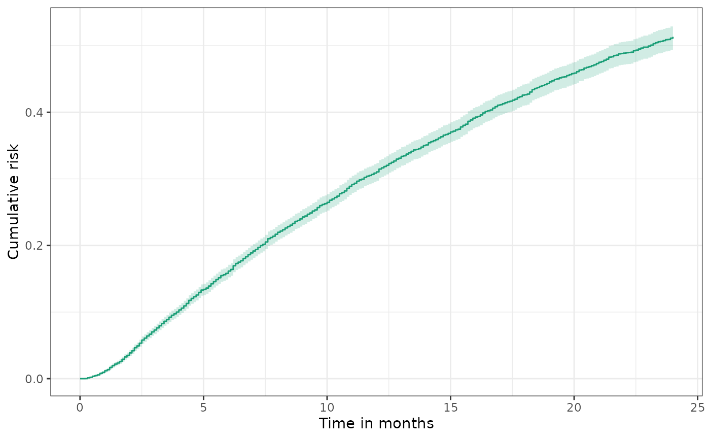
plot(fit2, effect_measure_type = "RD") +
  ylab("Cumulative risk difference") +
  xlab("Time in months")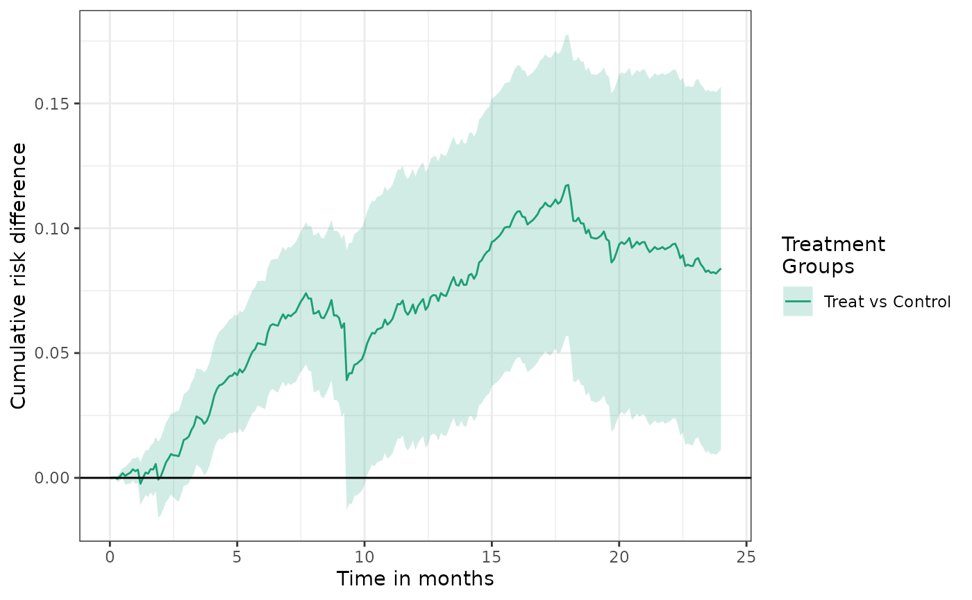

The cumulative risk ratio is often another important quantity of interest: \[ RR(t) = P(Y(1) < t) \;/\; P(Y(0) < t). \]

The plot function can produce a plot of the estimated cumulative risk ratio by setting the parameter effect_measure_type = "RR".

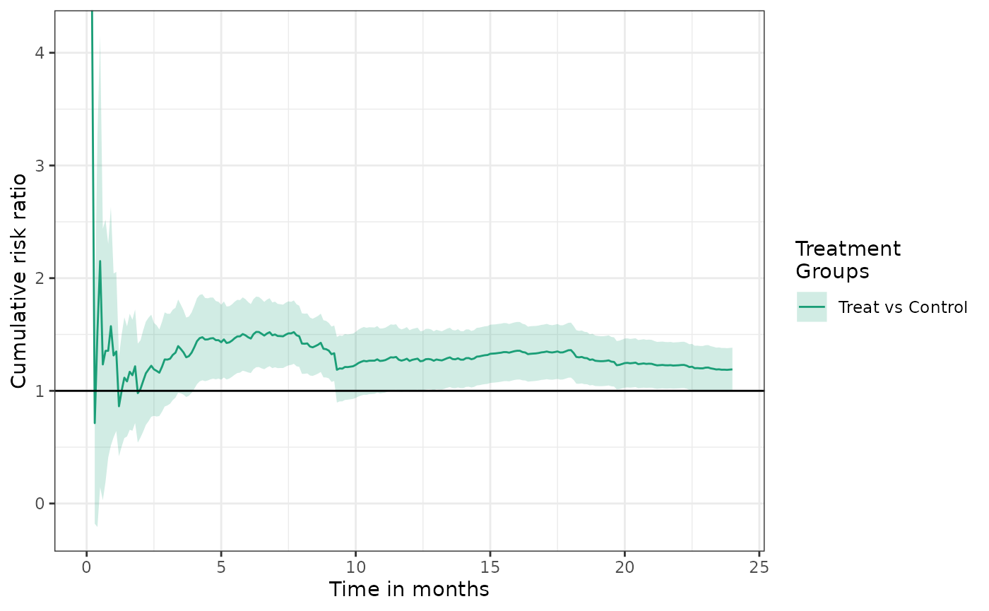
plot(fit2, effect_measure_type = "RR") + ylab("Cumulative risk ratio") +
  xlab("Time in months")

See the causalRisk plot object documentation for other available effect measures.

Table 2s for counterfactual cumulative risk and effect measures

Typical table 2 output can be generated by the function make_table2. This function reports the person-time of follow-up, events, and rates, as well as the cumulative risk and risk difference (by default), which are computed at a user-specified time point (given in the argument risk_time). The cumulative risk difference automatically uses the first level of treatment factor variable as the reference, but this can be changed using the argument ref.

make_table2(fit2, risk_time = 10, effect_measure_type = "RD")

We can change the effect measure provided in the table by specifying another value for effect_measure_type such as "RR" (for risk ratio). See the make_table2 object documentation for other available effect measures.

make_table2(fit2, risk_time = 10, effect_measure_type = "RR")

Assessing balance of confouders in an IPTW analysis

To assess the extent to which weighting achieves balance of key confounders, one may compute the inverse-probability of treatment-weighted means of baseline covariates by treatment group. The function make_table1 can be used to generate this table:

make_table1(fit2, DxRisk, Frailty, Sex, graph = TRUE)

Characteristic¹	Control n=9953.53	Treat n=9908.35
DxRisk, Mean (SD)	0.02 (0.97)	-0.03 (0.97)
Frailty, Mean (SD)	0.00 (1.00)	0.01 (0.99)
Sex
Female	4815 48.37	4769 48.13
Male	5139 51.63	5139 51.87
¹ All values are N (%) unless otherwise specified

Instead of providing the data and treatment, the function can also take as an argument the object that is returned by estimate_ipwrisk (or any that inherits from the ipw class), which contains the estimated weights and a reference to the data and subsetting conditions.

To assess balance, researchers often report standardized mean differences (SMDs). For continuous variables, the SMD between two groups is given as \[ d= \frac{\bar{X_i} - \bar{X_j}}{\sqrt{\frac{s^2_i+s^2_j}{2}}} \] where \(\bar{X_1}\) and \(\bar{X_2}\) and \(s^2_1\) and \(s^2_2\) are the sample means and variances of variable within each treatment group.

For dichotomous variables \[ d= \frac{\hat{p}_1 - \hat{p}_2}{\sqrt{\frac{\hat{p}_1(1-\hat{p}_1)+\hat{p}_2(1-\hat{p}_2)}{2}}} \] where \(\hat{p}_1\) and \(\hat{p}_2\) are the sample prevalences of the risk factors between the two treatment groups.

For categorical variables with \(k\) levels, we compute the SMD using the Mahalanobis distance. Let \[ G_1 = (\hat{p}_{1,2},\hat{p}_{1,3},\ldots,\hat{p}_{1,k})’ \] and \[ G_2 = (\hat{p}_{2,2},\hat{p}_{2,3},\ldots,\hat{p}_{2,k})’ \] where \(\hat{p}_{i,j}\) is the prevalence of level \(j\) in treatment group \(i\).

The standardized difference is given as \[ d = \sqrt{(G_1 - G_2) S^{-1}(G_1 - G_2)}, \] where \(S\) is a \((k-1)\) by \((k-1)\) covariance matrix with \[ S_{i,j} = \left\{ \begin{array}{c l} \frac{\hat{p}_{1,i}(1- \hat{p}_{1,i}) + \hat{p}_{2,i}(1- \hat{p}_{2,i})}{2}, & i = j\\ \frac{\hat{p}_{1,i}(\hat{p}_{1,j}) + \hat{p}_{2,i}(\hat{p}_{2,j})}{2}, & i \neq j \end{array}\right. \]

These statistics can be added to the table using the the option smd = TRUE:

make_table1(fit2, DxRisk, Frailty, Sex, smd = TRUE)

Characteristic¹	Control n=9953.53	Treat n=9908.35	SMD
DxRisk, Mean (SD)	0.02 (0.97)	-0.03 (0.97)	0.05
Frailty, Mean (SD)	0.00 (1.00)	0.01 (0.99)	-0.01
Sex			0
Female	4815 48.37	4769 48.13
Male	5139 51.63	5139 51.87
¹ All values are N (%) unless otherwise specified

Multiple censoring variables

Often researchers have data with multiple types of censoring. The package allows the analyst to create a composite of different types of censoring, combining together all types of censoring into a single variable. For example, with two censoring variables, denoted \(C_1\) and \(C_2\), we can estimate the cumulative risk using the following the estimating function: \[ \hat{Pr}(Y(a)<t)= \frac{1}{n}\sum_{i = 1}^{n} \frac{\Delta_{i} I(A_i=a)}{\hat{Pr}(\Delta=1|W_i,A_i, T_i) \hat{Pr}(A=a|W_i)}, \] where now \(\Delta=I(Y<C_1, Y<C_2)\) is an indicator that the patient was uncensored by the first and second type of censoring, respectively, and \(T = min(Y, C_1, C_2)\) is the earlier of the event or censoring times..

The estimating function depends again on two nuisance parameters: \(Pr(A=a|W)\), the propensity score or conditional probability of treatment and \(Pr(\Delta=1|W,A,T)\), the conditional probability that an observation will be uncensored by the first and second type of censoring at the observed minimum of their treatment and censoring times. As before, the current version of estimate_ipwrisk assumes a Cox proportional hazards model for the composite censoring variable.

In addition to the assumptions required for causal inference, the consistency of this estimating function requires that both \(C_1\) and \(C_2\) are conditionally independent of \((Y(a), a \in \mathcal{A})\) given \(W\) and that the model for \(Pr(\Delta=1|W, A, T)\) is correctly specified.

Estimation

To specify a model for these data, we can use the previously defined data structure, but add to it a second censoring variable. Note that the formula object for the first type of censoring is used to model the censoring risk of the composite.

models3 = specify_models(identify_treatment(Statin, formula = ~DxRisk),
                              identify_censoring(EndofEnrollment, formula = ~DxRisk),
                              identify_censoring(Discon),
                              identify_outcome(Death))

As before the model can be fit using the function estimate_ipwrisk

fit3 = estimate_ipwrisk(example1, models3, 
                   times = seq(0,24,0.1),
                   labels = c("IPTW+IPCW-2 main analysis"))

The table-making functions can accept multiple causalRisk objects, so we can tabulate the results from different analyses:

make_table2(fit2, fit3, risk_time = 10)

Competing risks analysis with counterfactual outcomes

The estimating functions for counterfactual risk can be extended to settings with competing risks. The counterfactual event time \(Y(a)\) is either the time of the competing event or the event of interest, whichever occurs first. We are first interested in estimating the cumulative risk that the event of interest has occurred first by time \(t\), or \(F_a(t)=P(Y(a)<t, J(a)=1)\), where \(J(a)\) is an indicator that \(Y(a)\) is the time of the event of interest, rather than the competing event. Note that the competing event indicator is indexed by \(a\) and is itself a counterfactual. \[ \hat{Pr}(Y(a)<t, J(a)=1)= \frac{1}{n}\sum_{i = 1}^{n} \frac{\Delta_{i} I(Y_i<t, J_{i}=1)I(A_{i}=a)}{\hat{Pr}(\Delta=1|W_i,A_i,T_i) \hat{Pr}(A=a|W_i)}, \] In addition to the assumptions required for causal inference, the consistency of this estimating function requires that both \(C_1\) and \(C_2\) are conditionally independent of \(\{(Y(a), J(a)), a \in \mathcal{A}\}\) given \(W\) and that the model for \(Pr(\Delta=1|W, A, T)\) is correctly specified.

Estimation

In the example data set, example1, the variable CvdDeath indicates whether Death is the event of interest or a competing event. To conduct a competing risks analysis, we can add to the data structure object a competing risk attribute. This is done with the constructor function identify_competing_risk, which depends on parameters event and event_value. The parameter name identifies the variable that indicates whether the outcome is the outcome of interest or a competing event; and event_value provides the value that the variable identified by name takes when the event is the event of interest rather than a competing event. In the data structure, we identify CvdDeath as the event indicator variables and indicate that CvdDeath=1 denotes the event of interest by specifying event_value = 1:

models3_cr1 = specify_models(identify_treatment(Statin, formula = ~DxRisk),
                              identify_censoring(EndofEnrollment, formula = ~DxRisk),
                              identify_censoring(Discon),
                              identify_competing_risk(name = CvdDeath, event_value = 1),
                              identify_outcome(Death))

As before the model can be fit using the function estimate_ipwrisk

fit3_cr1 = estimate_ipwrisk(example1, models3_cr1, 
                   times=seq(0,24,0.1),
                   label=c("CV mortality"))

In competing risks analysis, often one reports the cumulative incidence of the composite of both the competing event and the event of interest, alongside the cumulative incidence of the event of interest and the competing event computed separately.

models3_cr0 = specify_models(identify_treatment(Statin, formula = ~DxRisk),
                              identify_censoring(EndofEnrollment, formula = ~DxRisk),
                              identify_censoring(Discon),
                              identify_competing_risk(name = CvdDeath, event_value = 0),
                              identify_outcome(Death))

fit3_cr0 = estimate_ipwrisk(example1, models3_cr0,
                     times = seq(0,24,0.1),
                     labels = c("Non-CV mortality"))

plot(fit3, fit3_cr0, fit3_cr1, ncol=3, scales="fixed")

When the results of the different analyses are tabulated, the sum of the cumulative risk for each of the events should equal the cumulative risk of the composite event.

make_table2(fit3, fit3_cr0, fit3_cr1, risk_time = 10)

Estimating risk with more than two treatment groups

In many settings, researchers may be confronted with treatments that may have >2 levels. In our example data set, the treatment group can be further broken down into users of the high and low potency versions of treatment. The estimating functions described above can be straight-forwardly extended to multicategorical treatments, by estimating \(Pr(A=a|W)\) using a model appropriate for categorical outcomes with more than two levels. When the treatment variable identified in the data structure object is found to have >2 levels, estimate_ipwrisk estimates the treatment probabilities using multinomial logistic regression. However, other models can be used (see [Specifying alternative estimators]).

We can revise our analysis above to examine the risk associated with no treatment, low potency treatment, and high potency treatment by specifying StatinPotency to be our treatment in the data structure object:

models4 = specify_models(identify_treatment(StatinPotency, formula = ~DxRisk),
                              identify_censoring(EndofEnrollment, formula = ~DxRisk),
                              identify_censoring(Discon),
                              identify_competing_risk(name = CvdDeath, event_value = 1),
                              identify_outcome(Death))

fit4 = estimate_ipwrisk(example1, models4,
                   times = seq(0,24,0.1),
                   labels = c("Overall cumulative risk"))

The generic function plot, will produce the cumulative incidence functions for three treatment groups and confidence intervals:

plot(fit4) + ylab("Cumulative risk") +
  xlab("Time in months")

Risk difference plots can also be generated. By default the reference group is the first level of the treatment variable.

plot(fit4, effect_measure_type = "RD") +
  ylab("Cumulative risk") +
  xlab("Time in months")

In tables and plots, the reference group can changed by setting the ref parameter:

plot(fit4, effect_measure_type = "RD", ref = 2) +
  ylab("Cumulative risk") +
  xlab("Time in months")

Summarizing weights

One commonly encountered problem with inverse-probability of treatment weighted analyses is the occurrence of very large weights that give rise to highly variable and potentially biased estimators. Large weights occur when patients receive an apparently unlikely treatment. The causalRisk package contains a variety of functions that can be used to help diagnosis and address problems of large weights. The function make_wt_summary_table provide basic summary of treatment weights by treatment group:

make_wt_summary_table(fit2)

For standard IPTWs, the sum of the weights should be approximately equal to the overall sample size of the cohort. The existence of very large weights can reveal violations or near violations of positivity (i.e., the groups are fundamentally non-comparable).

The data on patients with large weights can be inspected using the function extreme_weights:

extreme_weights(fit2)

Propensity score distributions and trimming and truncation

Additional diagnostic information about IPTW analyses can be obtained by examining the propensity score distributions by treatment group. Such an analysis can reveal potential problems with non-positivity. The generic hist function will plot PS distributions by treatment group.

hist(fit2)

When areas of non-overlap exist, analysts often trim (drop) patients whose propensity score falls above or below a certain cut-point or truncating weights above a certain threshold.[9] Trimming can be implemented by setting the trim parameter in estimate_ipwrisk. The following function call trims all patients with a propensity score below 0.05 and above 0.95.

fit2_trim = estimate_ipwrisk(example1, models2, 
                   times = seq(0,24,0.1), 
                   trim = 0.05,
                   labels = c("IPTW+IPCW Main Analysis, Trimmed"))

hist(fit2, fit2_trim)

make_table1(fit2, DxRisk, Frailty, Sex)

Characteristic¹	Control n=9953.53	Treat n=9908.35
DxRisk, Mean (SD)	0.02 (0.97)	-0.03 (0.97)
Frailty, Mean (SD)	0.00 (1.00)	0.01 (0.99)
Sex
Female	4815 48.37	4769 48.13
Male	5139 51.63	5139 51.87
¹ All values are N (%) unless otherwise specified

make_table1(fit2_trim, DxRisk, Frailty, Sex)

Characteristic¹	Control n=8979.68	Treat n=8977.18
DxRisk, Mean (SD)	0.01 (0.78)	-0.01 (0.79)
Frailty, Mean (SD)	0.00 (1.01)	0.00 (1.00)
Sex
Female	4355 48.50	4340 48.34
Male	4625 51.51	4637 51.65
¹ All values are N (%) unless otherwise specified

In this case, trimming the top and bottom 5% of the populations by the propensity score, modestly reduces the population size and reduces the maximum weights and their variance.

make_wt_summary_table(fit2, fit2_trim)

However, trimming has only a modest effect on the estimated cumulative risks and risk difference.

make_table2(fit2, fit2_trim, risk_time = 10)

Truncation can be implemented by setting the trunc parameter in estimate_ipwrisk. The following function call truncates all weights above 95th percentile of the weight distribution (sets them equal to the 5th percentile).

fit2_trunc = estimate_ipwrisk(example1, models2, 
                   times = seq(0,24,0.1), 
                   trunc = 0.95,
                   labels = c("IPTW+IPCW Main Analysis, Truncated"))

hist(fit2, fit2_trim, fit2_trunc, ncol = 1)

In this case, truncating the propensity score at 5% and 95% reduces the maximum weights and their variance.

make_wt_summary_table(fit2, fit2_trunc)

In this case, truncation had a fairly substantial effect on the estimated cumulative risks and risk difference.

make_table2(fit2, fit2_trunc, risk_time = 10)

Standardized mortality ratio weights

Trimming the population on the propensity score may improve the internal validity of the analysis by reducing violations of the positivity assumption; however trimming changes the target population and therefore the results may not generalize to the population of interest. Also since the target population is now defined using the propensity score, an abstract quantity, the results will be less meaningful. In situations where there is little treatment effect heterogeneity across levels of the propensity score, the difference between these estimands is likely minimal. However, several studies have reported cases where trimming leads to substantial differences in point estimates. [10],[11]

Instead of trimming, analysts may also use alternative weighting schemes to target different populations. The so-called “standardized mortality ratio” (SMR) weight allows one to estimate treatment effects that generalize to the population represented by specific treatment groups.[12]

For example, in the case of a dichotomous treatment where patients are treated or untreated \((A \in \{0,1\})\), one could use an SMR weighting approach to estimate average effect of treatment in the treated (ATT): \[ RD(t) = P(Y(1) < t| A=1) - P(Y(0) < t|A=1). \]

The standard IPTW for two treatment groups (used in the previous estimating functions) is given by \[ w = \frac{I(A=a)}{Pr(A=a|W)} \] An SMR weight that standardizes the analysis to the treatment group \(A=1\) is given by \[ w_{1} = I(A=1) - I(A\neq 1) \frac{Pr(A=1|W)}{1-Pr(A=1|W)}. \] This yields a weight of one for patients with \(A=1\) and a weight equal to the propensity score odds of treatment (\(A=1\)) for patients with \(A=0\). The approach can be inverted to estimate the effect in the untreated or, for multicategorical treatments, any particular treatment group. We further standardize these weights to sum to \(n\) in each treatment group.

SMR weights can be requested by setting the wt_type parameter to identify the treatment group that should be used as the standard. The following code estimates the cumulative risk in each treatment group, re-weighting the patients in the treatment group (the second treatment group) in the example data set to be similar the patients in the control group.

fit2_smrw1 = estimate_ipwrisk(example1, 
                         models2, 
                         times = seq(0,24,0.1), 
                         wt_type = 1,
                         labels = c("IPTW+IPCW, standardized to Control"))

The weights can then be used to create an inverse-probability weighted table of means of baseline covariates.[13]

make_table1(fit2_smrw1, DxRisk, Frailty)

Characteristic¹	Control n=10000.00	Treat n=10000.00
DxRisk, Mean (SD)	0.74 (0.85)	0.67 (0.77)
Frailty, Mean (SD)	0.01 (1.02)	-0.01 (0.98)
¹ All values are N (%) unless otherwise specified

When compared to the unweighted means of covariates by treatment group, we can see that the means of DxRisk and Frailty in the group of patients in the control group are unchanged, but the means of covariates in the treatment group are now similar to the means in the control patients.

make_table1(example1, Statin, DxRisk, Frailty)

Characteristic¹	Control n=3201	Treat n=6799
DxRisk, Mean (SD)	0.74 (0.85)	-0.35 (0.88)
Frailty, Mean (SD)	0.01 (1.02)	0.02 (1.00)
¹ All values are N (%) unless otherwise specified

As before, the means in the weighted table can be used to assess the effectiveness of the weighting with respect to balancing the means of the baseline covariates (confounders).

Similarly, we could standardize the analysis to the second level of treatment (here Treatment) and estimate the effect of treatment in the population represented by those patients.

fit2_smrw2 = estimate_ipwrisk(example1, models2, 
                   times = seq(0,24,0.1), 
                   wt_type = 2,
                   labels = c("IPTW+IPCW, standardized to Treatment"))

Using these weights, the means of the covariates in the control group are now similar to the means in the treatment group.

make_table1(fit2_smrw2, DxRisk, Frailty)

Characteristic¹	Control n=10000.00	Treat n=10000.00
DxRisk, Mean (SD)	-0.32 (0.83)	-0.35 (0.88)
Frailty, Mean (SD)	0.00 (0.99)	0.02 (1.00)
¹ All values are N (%) unless otherwise specified

Examining the distribution of the PS in the unweighted and SMR weighted sample can also provide insight into how these weights are operating to affect the target population. In the overall population, we have the following distribution of PSs.

hist(fit2, by_treat = FALSE)

When these are stratified by treatment group, we see substantial differences between the groups.

hist(fit2)

When these distributions are weighted with IPT weights, we see that the PS distributions in both treatment groups looks like the distribution in the overall population.

hist(fit2, weight = TRUE)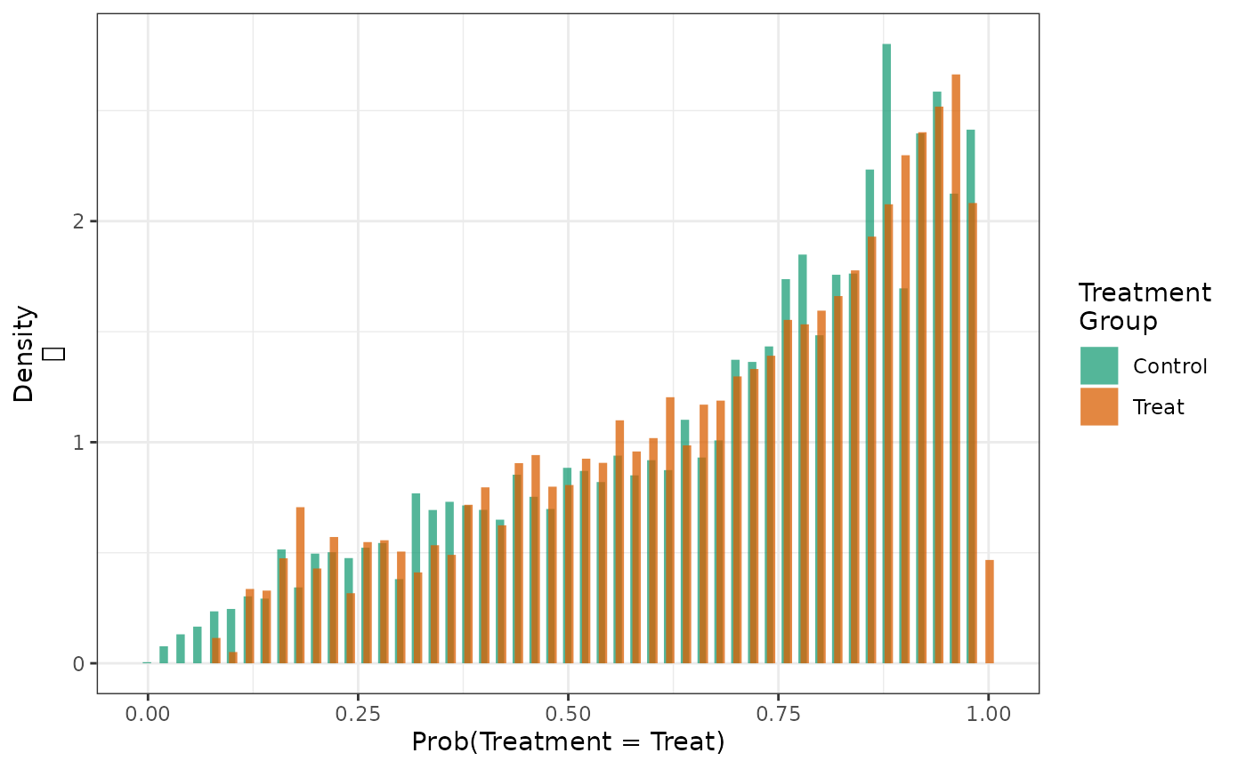

When the distributions are weighted with SMR weights standardizing to the control group, we see that the PS distributions in both treatment groups looks like the distribution in the untreated.

hist(fit2_smrw1, weight = TRUE)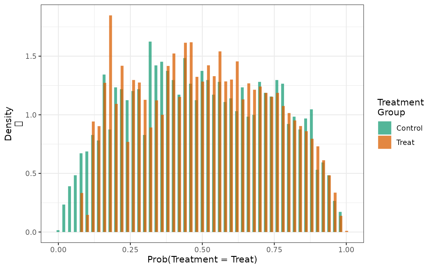

And the similar effect is observed when the distributions are weighted with SMR weights standardizing to the treated group.

hist(fit2_smrw2, weight = TRUE)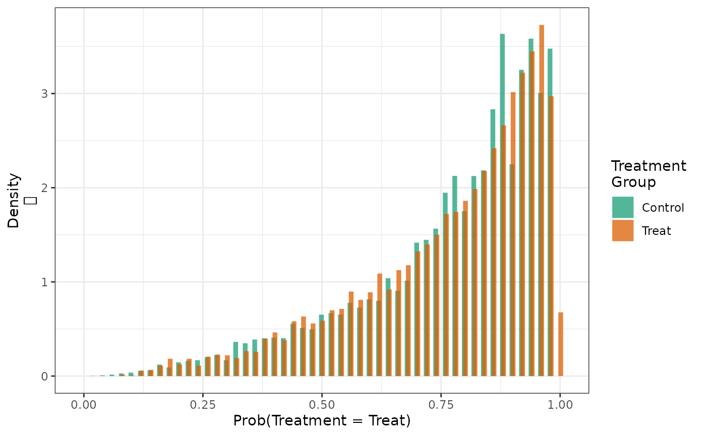

We can examine the variance and maximum values of the \(SMR\) weights in the treatment and control groups for each type of standardization. We see most variability in the weights in the control group when trying to standardize it to the treatment group, suggesting that there is relatively less information in the data to inform our estimate of what would happen to these patients if they were treated.

make_wt_summary_table(fit2, fit2_smrw1, fit2_smrw2)

In the simulated data, we see the effect of treatment in the group of patients typical of those receiving treatment appears to be smaller on the risk difference scale than the group representing those control patients.

make_table2(fit2, fit2_smrw1, fit2_smrw2, risk_time = 10)

Overlap Weights

Another alternative to trimming is to upweight individuals with propensity scores close to 0.5 and downweight individuals with propensity scores near 0 or 1 via an “overlap weight”.[14] To use overlap weights, specify wt_type = "o".

fit2_overlap = estimate_ipwrisk(example1, models2, 
                                times = seq(0,24,0.1), 
                                wt_type = "o",
                                labels = c("IPTW+IPCW, overlap weights"))

Looking at the distribution of the propensity scores after applying the overlap weights, we see that the treatment and control groups have nearly completely overlapping distributions, with the distribution being centered closer to 0.5 than the distribution after applying standard IPTW weights.

hist(fit2, fit2_overlap, weight = TRUE)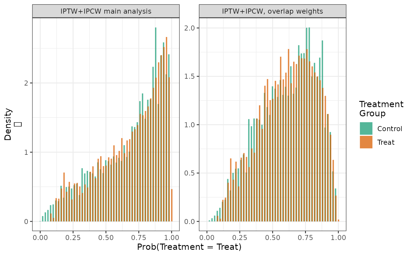

Comparing the estimates from the standard IPTW analysis to the overlap-weighted analysis, we see that the overlap weighted estimates of the risks and risk difference are less variable than the standard IPTW estimates. However, the estimates from the two approaches differ, as the target population is different for the two methods.

make_table2(fit2, fit2_overlap, risk_time = 24)

Like trimming, overlap weighting may improve the internal validity of the analysis by reducing violations of the positivity assumption. However, also like trimming, overlap weighting changes the target population and therefore the results may not generalize to the population of interest. Additionally, because the population after overlap weighting is defined by the distribution of the propensity scores, it can be difficult to identify the target population of the estimator.

Normalized weights

With standard inverse probability of treatment weights, it is possible for the sum of the weights to be substantially different from the size of the study population, particularly when there are near-positivity violations. This can lead to unstable estimates and large variances. One strategy to reduce the variance of the weights is to normalize them so that they sum to the population size. The normalized weights take the form: \[ w_{i,normalized} = w_{i,standard}\frac{n}{\sum_{j=1}^n w_{j,standard}} \]

To implement normalized weights in causalRisk, the user can specify wt_type = "n".

fit2_norm = estimate_ipwrisk(example1, 
                             models2, 
                             times = seq(0,24,0.1), 
                             wt_type = "n",
                             labels = c("IPTW+IPCW, Normalized Weights"))

We can compare the weight distributions between the standard and normalized weights. Notice that the sum of the normalized weights is exactly the size of the study population.

make_wt_summary_table(fit2, fit2_norm)

Next, we can compare the estimates using standard and normalized weights. Notice that the width of the confidence interval for the risk difference is smaller for the normalized-weights estimator, but the estimates remain similar.

make_table2(fit2, fit2_norm, risk_time = 24)

Stabilized Weights

When fitting marginal structural models with IPTW for time-varying treatments, it is often the case that the weights become very large as a result of few patients following each specific treatment history. A solution proposed by Robins et al. is to use stabilized weights. [15] Stabilized weights are similar to standard IPTW, but instead of using a numerator of 1, the numerator is the probability of following the specific treatment trajectory conditional only on baseline covariates. When stabilized weights are used in this case, the marginal structural model must condition on the baseline covariates, and the resulting estimate will be conditional on those covariates (it may seem paradoxical that a marginal structural model yields a conditional estimate, but the word “marginal” in “marginal structural model” has a distinct meaning, as explained by Breskin et al. [16]).

For single time-point exposures, stabilized weights are simply the standard IPTW multiplied by the marginal probability of exposure. \[ w_{i,stabilized} = w_{i,iptw}\times Pr(A=a) \]

When using stabilized weights, it is necessary to normalize the weights so that they sum to the total sample size. In fact, because \(Pr(A=a)\) is a constant, it cancels out when normalized, and the resulting estimates are exactly those of the estimator using the normalized weights.

Though the two methods, the IPTW with normalized weights and IPTW with stabilized weights, produce identical estimates, stabilized weights are still available to users of causalRisk. They can be used by specifying wt_type = "s".

fit2_stabilized = estimate_ipwrisk(example1, 
                                   models2, 
                                   times = seq(0,24,0.1), 
                                   wt_type = "s",
                                   labels = c("IPTW+IPCW, Stabilized Weights"))

When we compare the estimates, we notice that the they are exactly the same between the stabilized and normalized weights.

make_table2(fit2_norm, fit2_stabilized, risk_time = 24)

Diagnostics with more than two treatment groups

All of the package functions generalize to the situation with more than than two treatment groups.

make_table1(example1, StatinPotency, DxRisk, Frailty, Sex, graph = TRUE)

Characteristic¹	Control n=3201	Low Potency n=3393	High Potency n=3406
DxRisk, Mean (SD)	0.74 (0.85)	-0.35 (0.88)	-0.34 (0.87)
Frailty, Mean (SD)	0.01 (1.02)	0.01 (1.00)	0.03 (1.00)
Sex
Female	1581 49.39	1632 48.10	1655 48.59
Male	1620 50.61	1761 51.90	1751 51.41
¹ All values are N (%) unless otherwise specified

make_table1(fit4, DxRisk, Frailty, Sex, graph = TRUE)

Characteristic¹	Control n=9949.67	Low Potency n=9954.99	High Potency n=9863.86
DxRisk, Mean (SD)	0.02 (0.97)	-0.01 (0.98)	-0.04 (0.95)
Frailty, Mean (SD)	0.00 (1.00)	0.00 (1.00)	0.02 (0.99)
Sex
Female	4813 48.37	4753 47.74	4786 48.52
Male	5137 51.63	5202 52.26	5078 51.48
¹ All values are N (%) unless otherwise specified

make_wt_summary_table(fit4)

With more than 2 treatment groups, the propensity score now becomes a vector of probabilities that sum to one. To plot a PS histogram, one has to first select which probability to plot. We can do this using the cat option to the hist function. Using the results from the three group example presented previously, the following function call generates histograms of the probability that patients will be treated with the first treatment (the first value of the factor), which is labeled Control:

hist(fit4, cat = 1)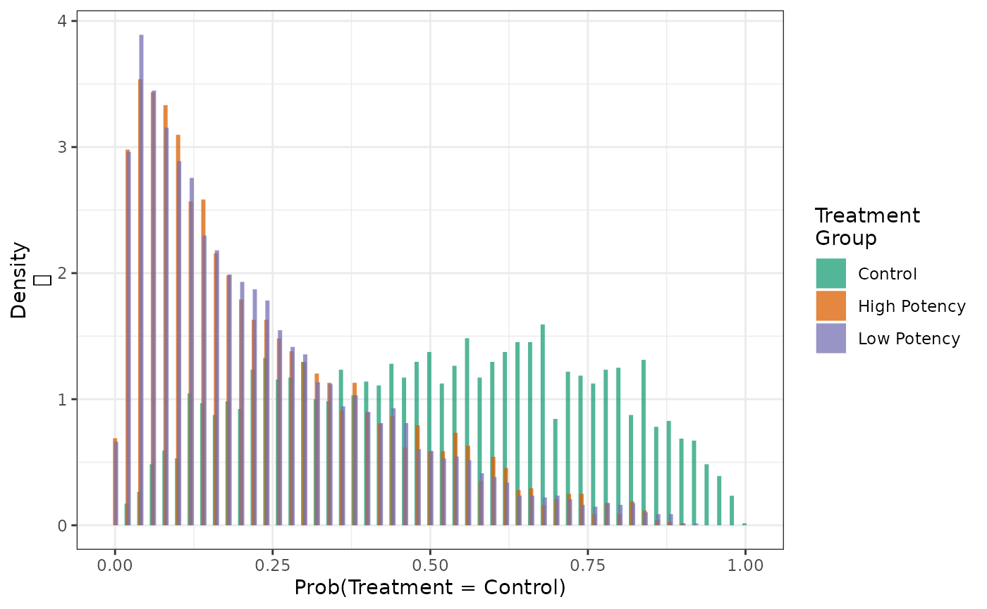

Similarly, we can examine the distribution of the probabilities that patients will be treated with the third category of treatment (the third value of the factor):

hist(fit4, cat = 3)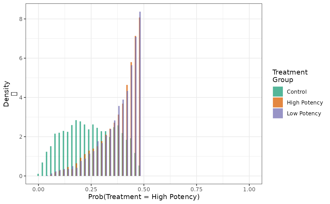

Bootstrap estimation

The default standard errors returned by estimate_ipwrisk are derived from the influence curve (or influence function) that assume known nuisance parameters. As discussed, these standard errors are tend to be conservative (too wide). When the nuisance models are estimated, the efficiency of the resulting estimator will increase slightly (or at worse, remain unchanged). This possible increase in efficiency is not captured in the influence curve-based estimated standard errors, as typically applied, therefore confidence intervals tend to be too wide.

More accurate confidence intervals can be obtained with a non-parametric bootstrap procedure. These can be obtaining by requesting bootstrap standard errors within the function estimate_ipwrisk:

fit2_boot = estimate_ipwrisk(example1, 
                             models2, 
                             times = seq(0,24,0.1), 
                             labels = c("Example1 -- Bootstrap"),
                             nboot = 250)

The parameter nboot sets the number of bootstrap iterations to be conducted. If a parallel back-end is registered, these computations will be done in parallel, if the parallel option is specified.

We can compare these different estimators by overlaying the risk difference plots:

plot(fit2, fit2_boot, rd = TRUE, overlay = TRUE) +
  ylab("Cumulative Risk Difference") + 
  xlab("Time in months")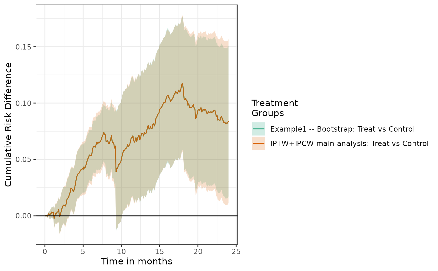

We can also tabulate the results, which suggest little difference in inference between the two approaches.

make_table2(fit2, fit2_boot, risk_time = 10)

Correlated data

In the presence of clustered/correlated data, for example multiple observations on a single subject, standard confidence intervals will be too narrow. A group-based bootstrap can be used to obtain valid confidence intervals. This approach is implemented in causalRisk. The user must request bootstrap standard errors and identify a subject identifier in the model specification object:

models_group = specify_models(identify_treatment(Statin, formula = ~DxRisk),
                              identify_censoring(EndofEnrollment, formula = ~Frailty + DxRisk),
                              identify_censoring(Discon),
                              identify_outcome(Death),
                              identify_competing_risk(name = CvdDeath, event_value = 1),
                              identify_subject(id))

When the data structure contains a subject identifier, the bootstrap procedure will automatically perform a group-based bootstrap, in which subjects and all their observations are resampled (for more details, see Technical Appendix)

Note bootstrap standard errors may not perform well when the size of the sample is very small.

Estimating counterfactual cumulative risk using an outcome model

The cumulative risk can also be estimated using an assumed outcome model, rather than assumed models for treatment and censoring. This estimator is a simple application of a parametric g-formula estimator for right censored data.[17] Here the analyst assumes a model for the conditional cumulative risk: \(Pr(Y<t|W,A)\). Given the fitted model, the counterfactual cumulative risk is then estimated with \[ \hat{Pr}(Y(a)<t)= \frac{1}{n}\sum_{i = 1}^{n} \hat{Pr}(Y<t|W_i,A=a), \] where \(\hat{Pr}(Y<t|W_i,A=a)\) is the predicted value of cumulative risk for patient \(i\) if treatment would have been \(A=a\). The causalRisk package implements such an estimator. The package estimates \(\hat{Pr}(Y<t|W,A)\) by fitting a Cox regression within each treatment group and then estimating subject-specific probabilities with a Breslow estimator.[18] The covariates contained in \(W\) should include all predictors of censoring and treatment that are also related to the outcome.

In order to implement this estimator, one needs to add a formula to the outcome object in the model specification

models_gcomp = specify_models(identify_treatment(Statin),
                        identify_censoring(EndofEnrollment),
                        identify_outcome(Death, ~DxRisk))

fit2_gcomp = estimate_gcomprisk(example1, 
                             models_gcomp,
                             times = seq(0,24,0.1), 
                             labels = c("Example1 -- G-computation"),
                             nboot = 25)

We see that the cumulative risks look similar to the IP weighted estimator; however, in this case the estimated risk and risk differences coming from the \(g\)-formula estimator have much smaller standard errors.

plot(fit2_boot, fit2_gcomp,  scales = "fixed")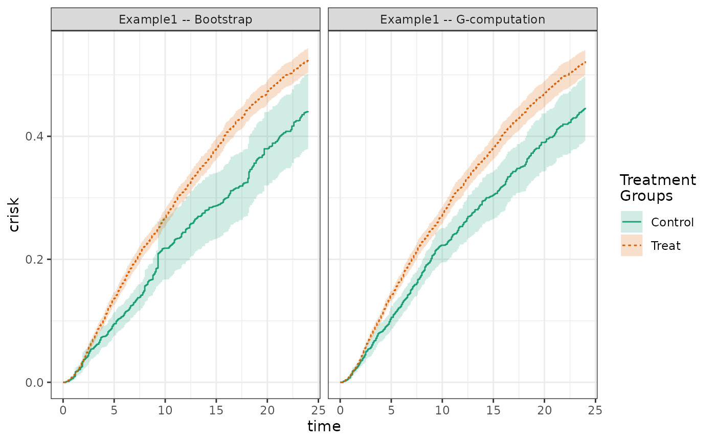

plot(fit2_boot, fit2_gcomp, rd = TRUE,  scales = "fixed")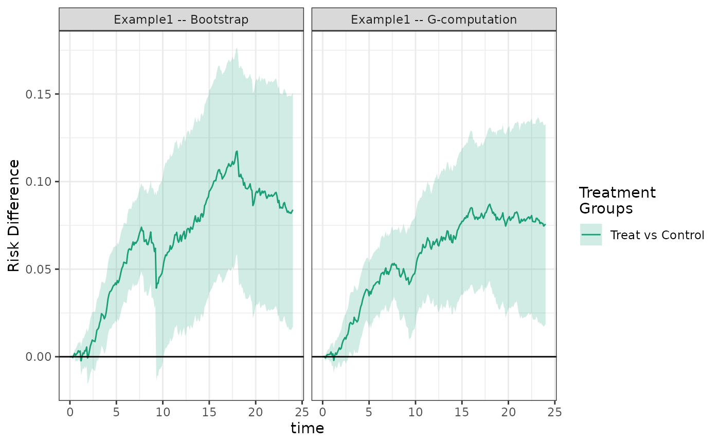

Note the \(g\)-formula estimator does not currently handle competing risks or missing data.

Estimating counterfactual cumulative risks using augmented inverse probability weighting

The augmented inverse probability weighted (AIPW) estimator uses models for both treatment/censoring (to produce weights) as well as a model for the outcome. In most cases, AIPW is more efficient than IPW, though less efficient than the \(g\)-formula estimator. AIPW has three other desirable properties

It is doubly robust, meaning that if either the treatment and censoring models or the outcome model is properly specified, the estimator remains consistent.
The influence curve based variance estimate is not conservative.
Valid inference is possible even when all of the models are fit with data adaptive machine learning methods.

causalRisk implements two AIPW estimators. Both handle competing risks. The first is a semiparametric efficient doubly robust estimator. [19] In this estimator, the counterfactual cumulative risk is then estimated with \[ \begin{aligned} &\hat{Pr}(Y(a)<t) = \frac{1}{n}\sum_{i = 1}^{n} \frac{\Delta_i I(Y_i<t, J=1) I(A_i=a)}{\hat{Pr}(\Delta=1|W_i,A_i,T_i) \hat{Pr}(A=a|W_i)} + \\\\ &\hat{Pr}(Y<t, J=1|A_i=a,W_i)\left(1-\frac{I(A_i=a)}{\hat{Pr}(A=a|W_i)}\right) + \frac{\hat{G}_iI(A_i=a)}{\hat{Pr}(A=a|W_i)} \\\\ \text{Where} \\\\ &\hat{G}_i = \int_0^{\tau_i} \frac{\hat{Pr}(Y<t,J=1|A_i,W_i)-\hat{Pr}(Y<k,J=1|A_i,W_i)}{1-\hat{Pr}(Y<k|A_i,W_i)}\frac{1}{\hat{Pr}(C_i>t|W_i,A_i)}d\hat{M}_i^C(k) \\\\ &M_i^C(k) = N_i^C(k) - \int_0^k I(Y_i \wedge C_i \ge s)\Lambda^C(ds|A_i,W_i) \\\\ &N_i^C(k) = I(Y_i \wedge C_i \le k, \Delta_i=0) \\\\ &\tau_i = min(Y_i, C_i, t) \end{aligned} \] and \(\Lambda^c(s|A, W)\) is the cumulative hazard function of the conditional probability of remaining uncensored. The package estimates each model as described in the previous sections, with the addition of \(\hat{Pr}(Y<t,J=1|A_i,W_i)\) being fit with a Fine and Gray model. [20]

The second estimator is computationally faster, but is not semiparametric efficient. Unlike the efficient estimator, this version does not incorporate all of the information from censored subjects. This estimator is: \[ \begin{aligned} &\hat{Pr}(Y(a)<t) = \frac{1}{n}\sum_{i = 1}^{n} \hat{Pr}(Y<t, J=1|A=a,W_i)+\frac{I(C_i>\tau_i) (I(Y_i<t,J_{i}=1)-\hat{Pr}(Y<t,J=1|A=a,W_i)) I(A_i=a)}{\hat{Pr}(C_i>\tau_i|W_i,A_i) \hat{Pr}(A=a|W_i)} \end{aligned} \]

In order to implement this estimator, one needs to have formulas for the outcome, treatment, and censoring objects in the model specification.

models_aipw = specify_models(identify_treatment(Statin, ~DxRisk),
                        identify_censoring(EndofEnrollment, ~DxRisk),
                        identify_outcome(Death, ~DxRisk))

fit_aipw = estimate_aipwrisk(example1, 
                             models_aipw,
                             times = 24,
                             labels = c("Example1 -- AIPW"))

We see that the cumulative risks look similar to the IP weighted and \(g\)-formula estimators; however, in this case the estimated risk and risk differences coming from the AIPW estimator have standard errors between the IPW and \(g\)-formula estimators.

make_table2(fit2_boot, fit2_gcomp,  fit_aipw, risk_time = 24)

The function estimate_aipwrisk uses the fast, not semiparametric efficient estimator by default. To use the semiparametric efficient, but computationally more intensive, estimator, specify fully_efficient = TRUE in the function call. We recommend only using the efficient estimator on single time points due to the computational requirements.

Estimating the risk ratio and other measures of effect

The risk difference is a measure of effect that is easily interpreted and meaningful to clinicians and policy makers. However, in some cases alternative measures of effect may be desired. For example, interest often centers on the risk ratio \[ RR(t) = \frac{P(Y(1) < t)}{P(Y(0) < t)}. \] In the causalRisk package relative risk estimates can be added to table 2 output:

make_table2(fit2, fit2_boot, risk_time = 10, effect_measure_type = "RR")

Graphs of the relative risk can also be generated:

plot(fit2, fit2_boot, effect_measure_type = "RR") + ylab("Cumulative Relative Risk") + 
  xlab("Time in months")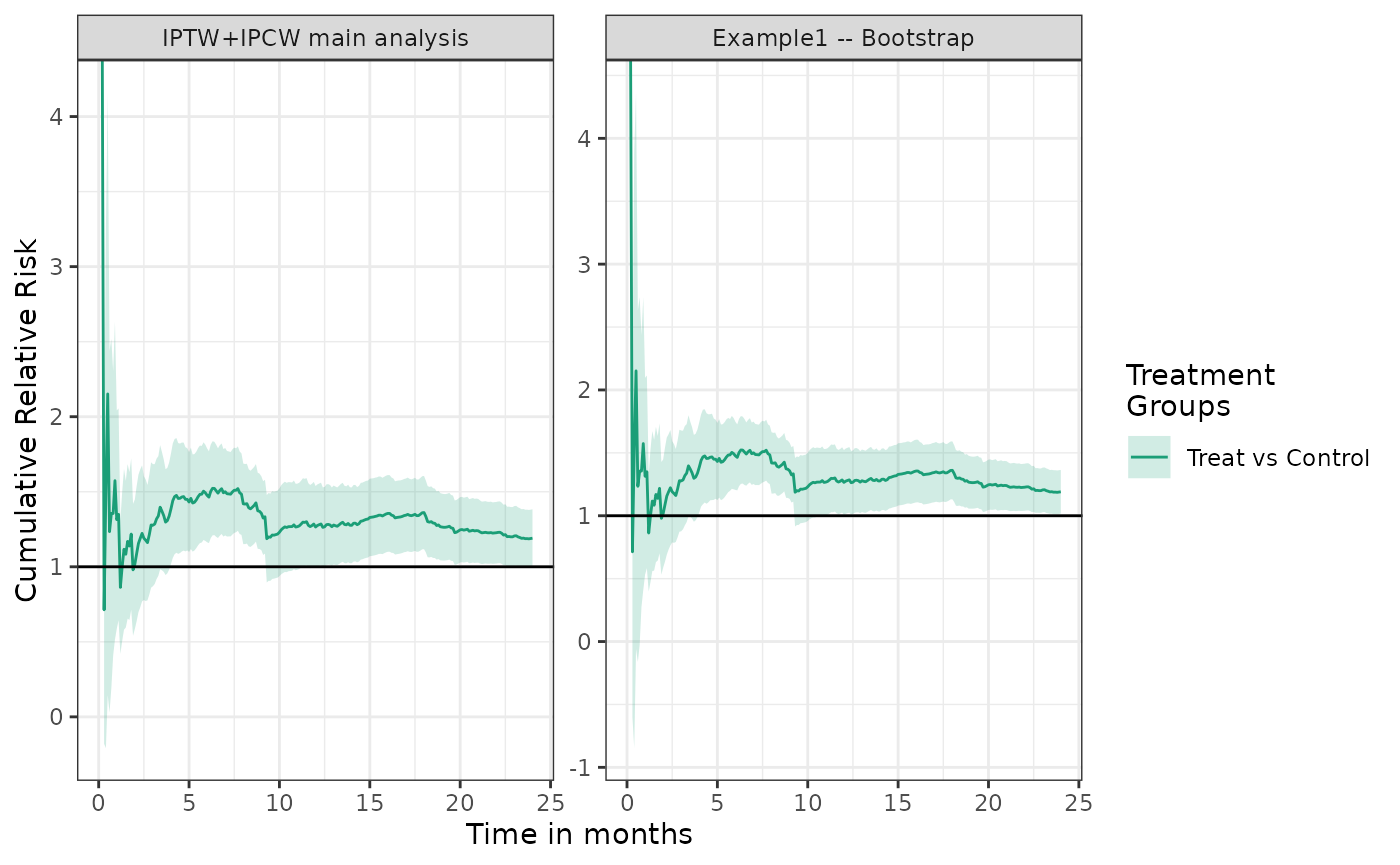

Expressive analysis pipeline

The causalRisk package aims to provide tools that allow common analysis tasks to be expressed simply, with unnecessary details abstracted away. For example, if we were interested in examining how the results of an analysis would change if a variable were taken out of the propensity score model, we could express this analysis as follows:

# what happens when we take DxRisk out of PS ?
fit2 %>%
  update_treatment(new_formula = ~.-DxRisk) %>%
  update_label("Drop DxRisk from PS") %>%
  re_estimate ->
  sens1

The %>% operator (from the magrittr package contained in tidyverse ) pipes output from one function into another. Here the original analysis is piped into the function update_a, which updates information about the treatment node in the data structure; here the function removes DxRisk from the treatment model. The function update_label, changes the label of the analysis and then the function re_estimate, re-estimates the cumulative risk with the change.

Similarly, we could examine how the results would be affected if Frailty were to be added to the propensity score:

# what happens when we add Frailty to the PS ?
fit2 %>%
  update_treatment(new_formula = ~.+Frailty) %>%
  update_label("Add Frailty to PS") %>%
  re_estimate ->
  sens2

plot(fit2, sens1, sens2, ncol = 3, scales = "fixed")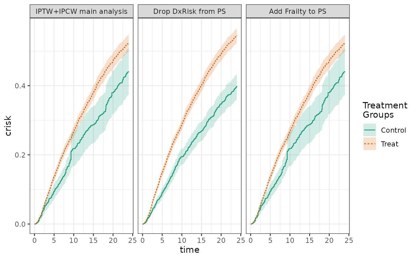

Compact expression of subgroup analyses

Subgroup analyses can also be expressed naturally using such pipeline approaches. The subgroup function in the causalRisk package can be used to repeat an analysis within a particular subgroup. The following code creates an adjusted analysis of StatinPotency by replacing the treatment Statin with StatinPotency in a previous adjusted analysis. The code then creates an unadjusted analysis by removing all variables in the treatment model. The code then specifies four subgroup analyses. The cumulative risk and risk difference curves are panel plotted for all analyses.

adj = fit2 %>%
  update_treatment(new_name = StatinPotency) %>%
  update_label("Adjusted") %>% re_estimate()

unadj = adj %>%
  update_treatment(new_formula = ~1) %>%
  update_label("Unadjusted") %>% re_estimate() 

not_frail = adj %>% subgroup(Frailty > 0) %>%
  update_label("Not Frail") %>% re_estimate()

frail = adj %>% subgroup(Frailty <= 0) %>%
  update_label("Frail") %>% re_estimate()

high_risk = adj %>% subgroup(DxRisk <= 0) %>%
  update_label("High Risk") %>% re_estimate()

low_risk = adj %>% subgroup(DxRisk > 0) %>%
  update_label("Low Risk") %>% re_estimate()

plot(unadj, adj, not_frail, frail, low_risk, high_risk, 
     scales = "fixed", ncol = 2) + 
  ylab("Cumulative Risk") + 
  xlab("Time in months")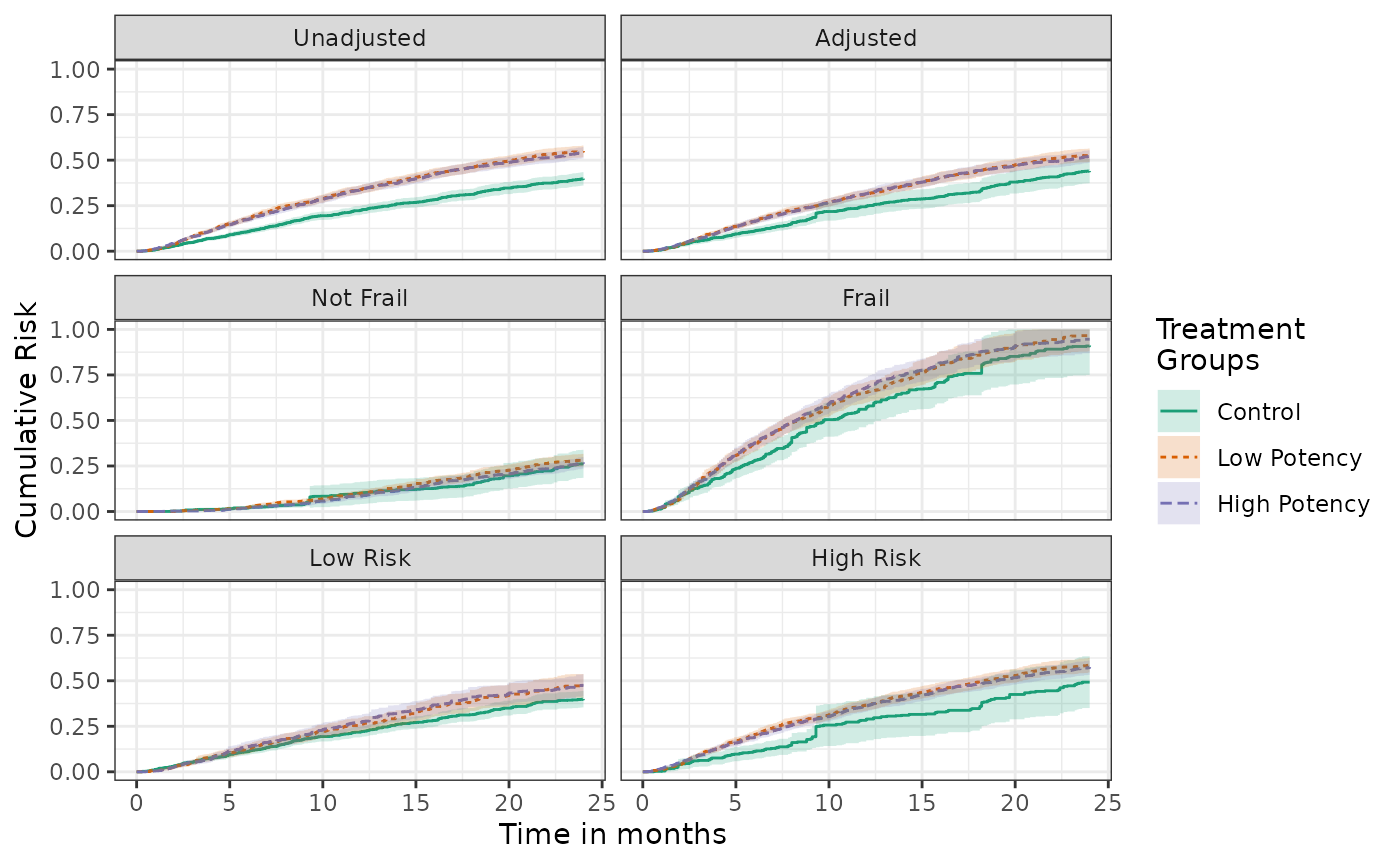

plot(unadj, adj, not_frail, frail, low_risk, high_risk, effect_measure_type = "RD", scales = "fixed", ncol = 2) + 
  ylab("Cumulative Risk Difference") + 
  xlab("Time in months")

When many subgroup analyses are specified, panel plots of the risk or risk difference curves may contain too much information to be easily interpreted. It may be easier to communicate the results via forest plots or cumulative risks, risk differences, or risk ratios at specific times points.

forest_plot(unadj, adj, not_frail, frail, low_risk, high_risk,  risk_time = 20)

forest_plot(unadj, adj, not_frail, frail, low_risk, high_risk, 
            effect_measure_type = "RD", risk_time = 20)

forest_plot(unadj, adj, not_frail, frail, low_risk, high_risk, 
            effect_measure_type = "RR", risk_time = 20)

Modeling censoring as a function of time-varying covariates

The package also allows the user to incorporate time-varying covariates into the censoring model. This is allows the risk of censoring to depend on both baseline covariates as well as events that occur during follow-up.

Now in the estimation functions, the risk of censoring depends on a covariate process, rather than just on covariate measured at baseline. To estimate counterfactual risk with a single censoring event, we can use the following estimating function: \[ \hat{Pr}(Y(a)<t)= \frac{1}{n}\sum_{i = 1}^{n} \frac{\Delta_i I(Y_i<t) I(A_i=a)}{\hat{Pr}(\Delta=1|\bar{W}_i(T_i),A_i, T_i) \hat{Pr}(A=a|W_i)}, \] where \(Y\) is the observed event time, \(C\) is the observed censoring time, \(T = \min(C,Y)\), \(\Delta = I(Y<C)\) is an indicator that the patient was uncensored, \(\bar{W}_i(T)\) is the history of the covariate process up until censoring or the outcome, and \(A\) is the observed treatment.

Data structure for time-varying covariates

To do this, the incoming data needs to include separate rows for each patient-interval under observation. Each observation should include the start and stop time of the interval. The first interval should start at zero. Intervals with no observed end time can be set to NA. Event times and censoring times can be specified as before, as days until the event occurs or NA if the event is not observed. An event or censoring variable that is either NA or larger than the first observed event or censoring time is taken to be censored at the first observation time.

The package is designed so that the required format of the incoming data requires minimal data processing to create. Censoring and event indicators are created by the estimation functions in causalRisk.

The package contains one example simulated data set with time varying covariates for illustration. The first twenty rows of this example data set example1_timevar appear below (routed through the table rendering function kable):

example1_timevar[1:20, ] %>% kable

id	DxRisk	Frailty	Sex	Statin	StatinPotency	EndofEnrollment	Death	Discon	CvdDeath	Interval	Start	Stop
1	0.933	-0.399	Male	Control	Control	2.316	NA	NA	NA	1	0	10
2	-0.525	-0.006	Female	Treat	Low Potency	0.210	NA	NA	NA	1	0	10
3	1.814	0.180	Male	Control	Control	6.629	NA	1.438	NA	1	0	10
4	0.083	0.388	Female	Treat	Low Potency	NA	34.2	16.215	1	1	0	10
4	0.903	0.388	Female	Treat	Low Potency	NA	34.2	16.215	1	2	10	NA
5	0.396	-1.111	Male	Treat	High Potency	3.919	NA	NA	NA	1	0	10
6	-2.194	-1.030	Female	Treat	Low Potency	2.189	NA	0.102	NA	1	0	10
7	-0.360	0.582	Male	Control	Control	0.134	NA	NA	NA	1	0	10
8	0.143	1.263	Male	Control	Control	14.555	NA	0.165	NA	1	0	10
8	-0.017	1.263	Male	Control	Control	14.555	NA	0.165	NA	2	10	NA
9	-0.204	-0.591	Male	Treat	Low Potency	NA	17.2	NA	0	1	0	10
9	0.414	-0.591	Male	Treat	Low Potency	NA	17.2	NA	0	2	10	NA
10	0.446	-0.730	Female	Control	Control	0.400	NA	NA	NA	1	0	10
11	-0.322	1.317	Female	Treat	Low Potency	16.909	NA	6.065	NA	1	0	10
11	-0.190	1.317	Female	Treat	Low Potency	16.909	NA	6.065	NA	2	10	NA
12	0.478	1.372	Female	Treat	High Potency	1.598	NA	NA	NA	1	0	10
13	0.196	-0.736	Male	Treat	Low Potency	0.106	NA	NA	NA	1	0	10
14	0.715	-0.212	Female	Control	Control	NA	15.5	NA	0	1	0	10
14	1.409	-0.212	Female	Control	Control	NA	15.5	NA	0	2	10	NA
15	-0.960	-1.145	Male	Treat	High Potency	NA	5.4	2.781	0	1	0	10

As with example1, the simulated data again come from our hypothetical cohort study designed to look at the effectiveness of statins in a routine care population with elevated lipids. Here the difference from the previous example data is that all patient surviving and uncensored at 10 months are followed up for additional measurement of the variable DxRisk. No additional measurement are made. Therefore each patient may contribute up to 2 records for the analysis dataset.

Describing the structure and models for data with time-varying covariates

The model specification for data with time-varying covariates is nearly identical as before, except the user must specify the variables that denote the start and stop of the intervals. This is done with the data descriptor function identify_interval. Also the user must identify a variable that denotes a subject identifier with the data descriptor function identify_subject.

timevar_models = specify_models(
  identify_interval(Start, Stop),
  identify_subject(id),
  identify_treatment(Statin, ~DxRisk),
  identify_censoring(EndofEnrollment, ~Frailty),
  identify_outcome(Death)
  )

The IP weighted estimating function for cumulative risk is invoked also via the function call estimate_ipwrisk:

timevar_results = estimate_ipwrisk(example1_timevar, 
                      timevar_models,
                      times = seq(0,24,0.1),
                      labels = c("Overall cumulative risk"))

plot(timevar_results)

Estimation of Cumulative Counts

In addition to estimating cumulative risk functions, the package is also able to estimate cumulative counts, such as counts of events or costs over time. The estimator is based off of the so-called ‘partitioned’ count estimator, with modifications to allow for counterfactual counts and informative censoring.[21] The general form of the cumulative count estimator used by the package is: \[ \hat{E}(Y(a))= \frac{1}{n}\sum_{i = 1}^{n} \sum_{k=1}^{t} \frac{I(A_i=a)\Delta_{i,k}Y_{i,k}}{\hat{Pr}(\Delta_k=1|\bar{W}_i(k),A_i) \hat{Pr}(A=a|W_i)}, \] where \(Y_k\) is the observed count occurring between times \(k-1\) and \(k\), \(C\) is the observed censoring time, \(\Delta_k = I(k<C)\) is an indicator that the patient was uncensored at time \(k\), \(\bar{W}_i(k)\) is the history of the covariate process up until time \(k\), and \(A\) is the observed treatment.

Data structure for cumulative count estimation

Incoming data for cumulative count estimation look similar to data for risk estimation with time-varying covariates. The incoming data needs to include separate rows for each patient-interval under observation. Each observation should include the start and stop time of the interval. The first interval should start at zero. Associated with each interval should be a variable representing the count that occurred during that interval.

Censoring times can be specified as before, as days until censoring occurs or NA if the censoring is not observed. Each row for an individual should include their censoring time(s), which should not change across rows.

Competing events are recorded as the time to competing event or NA if the competing event does not occur. If there are multiple competing events, they should be combined into a single variable indicating the earliest time. Each row for an individual should include their competing event time, which should not change across rows. As competing events preclude the accumulation of counts, no intervals should occur after the competing event.

Intervals should be non-overlapping, but must cover a continuous period of time (there cannot be gaps). The time period covered does not need to extend to the end of the study period, as internal functions will properly handle the person-time accrued by each subject.

New intervals should occur whenever a time-varying covariate changes value, even if no count occurs during that interval (the count for such intervals should simply be set to 0).

The package is designed so that the required format of the incoming data requires minimal data processing to create. Censoring indicators are created by the estimation functions in causalRisk.

The package contains one example simulated data set for cumulative count for illustration. The first twenty rows of this example data set example4 appear below (routed through the table rendering function kable):

example4[1:20, ] %>% kable

id	Interval	Start	Stop	Count	DxRisk	Sex	Statin	EndofEnrollment	Death
1	1	0.000	0.931	0	0.971	Male	Control	2.32	NA
2	1	0.000	0.426	2	-0.566	Female	Treat	0.21	NA
2	2	0.426	10.588	9	-0.405	Female	Treat	0.21	NA
2	3	10.588	14.532	9	-0.320	Female	Treat	0.21	NA
2	4	14.532	21.265	9	-0.094	Female	Treat	0.21	NA
2	5	21.265	23.245	0	-0.357	Female	Treat	0.21	NA
3	1	0.000	0.241	4	1.712	Male	Control	6.63	NA
3	2	0.241	2.859	0	1.892	Male	Control	6.63	NA
3	3	2.859	13.859	4	2.052	Male	Control	6.63	NA
4	1	0.000	9.723	6	0.344	Female	Treat	NA	34.2
4	2	9.723	17.367	4	0.090	Female	Treat	NA	34.2
5	1	0.000	4.625	3	0.729	Male	Treat	3.92	NA
5	2	4.625	5.998	5	0.639	Male	Treat	3.92	NA
5	3	5.998	39.159	1	0.716	Male	Treat	3.92	NA
5	4	39.159	40.420	7	0.813	Male	Treat	3.92	NA
5	5	40.420	43.122	2	0.768	Male	Treat	3.92	NA
5	6	43.122	44.545	5	0.597	Male	Treat	3.92	NA
5	7	44.545	47.279	4	0.797	Male	Treat	3.92	NA
6	1	0.000	0.178	8	-1.945	Female	Treat	2.19	NA
6	2	0.178	0.301	7	-1.941	Female	Treat	2.19	NA

The simulated data again come from our hypothetical cohort study designed to look at the effect of statins on costs due to hospitalizations over time. Each individual can contribute multiple rows, with each row corresponding to an interval during which an individual accrued costs due to hospitalizations or to a change in the DxRisk variable.

Describing the structure and models for cumulative count estimation

The model specification for cumulative count estimation is nearly the same as for cumulative risk estimation with time-varying covariates. The primary difference is the data descriptor function identify_outcome is replaced by the function identify_count. Competing events are identified using identify_outcome.

count_models = specify_models(
  identify_interval(Start, Stop),
  identify_subject(id),
  identify_treatment(Statin, ~DxRisk),
  identify_censoring(EndofEnrollment, ~DxRisk),
  identify_outcome(Death),
  identify_count(Count)
  )

The IP weighted estimating function for cumulative counts is invoked also via the function call estimate_ipwcount:

count_results = estimate_ipwcount(example4, 
                      count_models,
                      times = seq(0,24,0.1),
                      labels = c("Overall cumulative count"))

All of the same table and plot functions work for cumulative count estimation, for instance:

Table 1:

make_table1(count_results, DxRisk)

Characteristic¹	Control n=9169.86	Treat n=9168.50
DxRisk, Mean (SD)	0.25 (0.98)	0.20 (0.99)
¹ All values are N (%) unless otherwise specified

Propensity score histogram:

hist(count_results)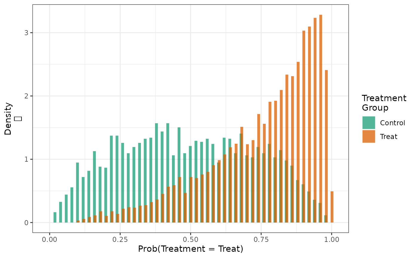

Cumulative count plot:

plot(count_results)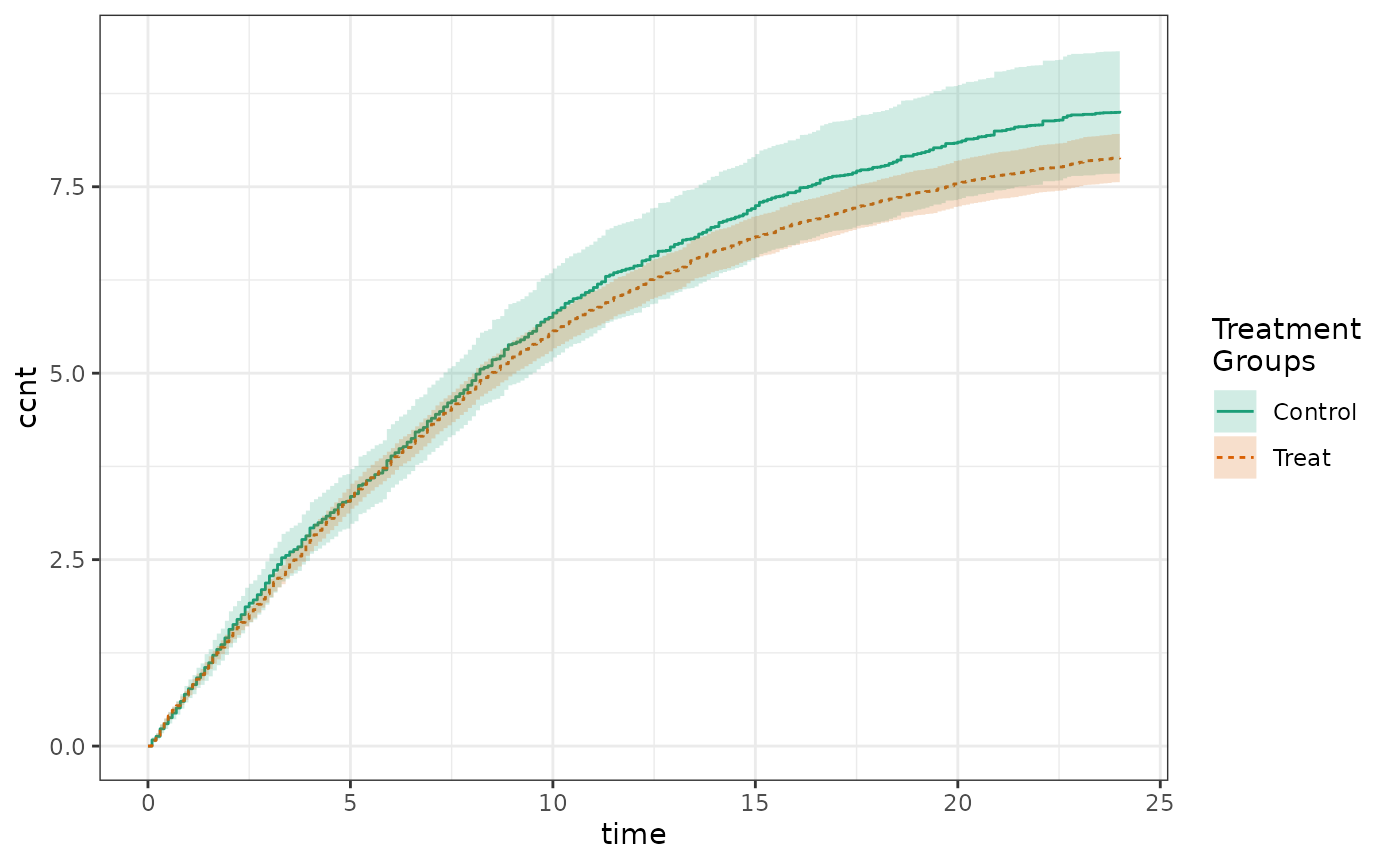

Summary results in a Table 2:

make_table2(count_results, count_time = 24)

Cumulative count estimation is also amenable to the expressive analysis pipelines previously described, and confidence intervals can be estimated using either the empirical influence function method or the bootstrap.

Technical appendix

Assumptions needed for causal inference

The estimators of causal effects described here require special assumptions. Although there are different sets of identification conditions for causal effects, here we focus on a core set of assumptions that have been frequently used to support the use of the semiparametric estimators described in this paper.

First we need that the interventions are well-defined and can be linked to observed treatments. This is often described as the consistency assumption. For treatment groups, consistency asserts that \(Y = I(A=1)Y(1) + I(A=0)Y(0)\). Alternatively, one can assume treatment version irrelevance, which states that different forms of the treatment are equivalent.[22] For example, the intervention that we wish to study might be the assignment of a patient to take 10mg atorvastatin daily at bedtime; however, we instead only observe that a patient started filling a prescription for atorvastatin. The assumption of treatment version irrelevance would assert that these different forms of treatment are equivalent.
Second, we assume that there is no interference between patients. This means that one patient’s treatment will not affect another patient’s outcome.[23] Interference is a concern in studies of treatments for infectious disease, such as vaccines. Consistency and no interference are sometime combined into a single assumption termed the “stable unit treatment value assumption” (SUTVA).
Third, we also need that there are no unmeasured confounders for treatment. This assumption is sometimes termed conditional exchangeability. Within levels of the confounders we want for treatment to be effectively randomized. This can be formalized as follows: \[ Y(a)\perp A | W, a \in \mathcal{A}, \] where \(\mathcal{A}\) is the set of treatments under consideration.
Fourth, we require positivity or equivalently the experimental treatment assignment assumption, which asserts that all patients have a non-zero probability of receiving any particular treatment being studied.[24] This can be expressed formally as: \[ \max_{a \in \mathcal{A}} |1/Pr(A=a|W)| < \infty, \] almost everywhere. Intuitively, if a certain patient subgroup in the target population is never treated, we cannot estimate the average effect of treatment in that population without making an assumption about treatment effect homogeneity.
Fifth, we assume no measurement error on exposure, confounders, or outcome.
Sixth, if the data are censored, we assume the counterfactual outcome are conditionally independent of the censoring variables given the baseline covariates.
Seventh, if data are missing, we make the stratified missing completely at random assumption. This means that, within strata of the completely measured variables, the data are missing completely at random. We note that this is a stronger condition than the missing at random assumption needed for imputation-based methods.
Finally, we assume correct specification of all statistical models.

Estimating standard errors with the influence curve

For the IP weighted estimators, the default confidence intervals reported by the software are conservative confidence intervals derived from the influence curve in which the nuisance parameters are taken to be known. These are computed from the variance of this influence function: \[ \hat{\sigma^2} = \frac{1}{n}\sum_{i = 1}^{n} [\hat{IC}(X_i;g)]^2 \] where the estimated influence curve for an observation is given by \[ \hat{IC}(X_i;g) = D(X_i;g) - \hat{F(t)} \] where \(X_i\) is observed data for patient \(i\), and \(g\) represents nuisance parameters, such as the propensity score, that are estimated using assumed models, and \(D(X_i;g)\) is a subjects contribution to the estimating function, e.g., \[ D(X_i;g) =\frac{\Delta_{i} I(Y_i<t)}{\hat{Pr}(\Delta_{i}=1|W_i)}. \]

We report asymptotic 95% confidence intervals using a normal approximation \[ \hat{Pr}(Y<t) \pm 1.96 \frac{\hat{\sigma}}{\sqrt{n}}, \] with the the upper and lower bound of the interval truncated at 0 and 1.

These confidence intervals assume that the nuisance parameters are known. However, in most situations they are unknown and must be estimated. Somewhat counter-intuitively, the estimation of nuisance parameters increases the efficiency of estimators.[3] For example, estimation of propensity scores results in improvements in efficiency over using a known propensity score,[25] provided the PS only contains variables that are related to the outcome.[26] Because of this phenomenon, the standard errors returned by the software will be conservatively biased (too large).

Note that these variance estimators assumes that the data are independent. Correct inference in the presence of dependent data needs to be addressed using the group-based bootstrap procedure included in the package.

Appendix

Handling tied event times

Tied event times are handled by breaking the ties subtracting a small random error (less than \(10^{-3}\)) off of each tied event time. By making this delta sufficiently small, we ensure that we will not cause any observed event to be censored and therefore the risk at the point of the tied event times will be correctly estimated. We add a small random error of the same magnitude to tied censoring times.

Bootstrap implementation

Currently, the bootstrap is implemented by an iterative re-weighting of the data within each cycle of the bootstrap algorithm. A non-parametric bootstrap would correspond to weighting the data with a vector of weights drawn from a multinomial distribution with size \(n\) and category probabilities given by \(p_i = 1/n, i=1, 2,\ldots,n\). To avoid problems with zero weights (which are not accepted by some estimation functions), we re-weight observations using a continuous (fractional) random weight drawn from a exponential distribution with mean 1.[27] The weights are then normalized to sum to \(n\). It has been shown that fractionally-weighted bootstrap estimators have good properties if positive independent and identically distributed weights are generated from a continuous distribution that has a mean and standard deviation equal to one. When subject_id is specified in the data structure object and a bootstrap confidence interval is requested, a group-based bootstrap is conducted in which clusters of observations, rather than patients, are weighted. Bootstrap confidence intervals are computed using the standard deviation of the bootstrap distribution as an estimate of the standard error: \(\hat{P}\pm Z_{1-\alpha/2} \hat{SE}(\hat{P})\).

S3 class definitions in `causalRisk`

The S3 classes defined in causalRisk are meant to be general enough to permit the expansion of the package to allow for the estimation of different parameters and also to permit the use of different estimating approaches, such the parametric \(g\)-formula, and augmented inverse-probability weighted estimators.

We define a variety of classes to describe objects that contain the results of estimation. These classes can identify both the estimand (parameter of interest) and the way that is was estimated. Currently the following classes are defined:

result all results objects generated by the package are assigned to be members of this class, although at present no specific methods are defined for it.
cumrisk indicates that the estimand is a cumulative risk curve; additional estimands are planned. The functions that plot and tabulate results are specific to what is being estimated. Different estimands will require different plotting methods and will need to be summarized using different types of tables.
ipw indicates that the parameter of interest is estimated using inverse-probability weighted estimating functions. The functions that summarize the weights and propensity scores are methods for classes of this type. Weights and propensity scores for all estimands can be summarized using the methods.
boot_est indicates that the parameter of interest was estimated using bootstrap estimation. The resulting object will contain a list of lists named boot_results. Each element in this list is the complete sets of results generated from each bootstrap iteration. The results will depend on what is being estimated. For a cumrisk object, the results consist of a set of cumulative risk curves one for each treatment group, and a table with the observed person time and rates, one row for each treatment group.

References

1. Laan MJ van der, Robins JM. Unified methods for censored and longitudinal data and causality. New York.: Springer Verlag; 2002.

2. Brookhart MA. Counterpoint: The treatment decision design. American Journal of Epidemiology. 2015;182.

3. Robins JM, Rotnitzky A. Recovery of information and adjustment for dependent censoring using surrogate markers. In: AIDS epidemiology-methodological issues. Jewell, N. Dietz, K.; 1992.

4. Hubbard AE, Laan MJ van der, Robins JM. Nonparametric locally efficient estimation of the treatment specific survival distribution with right censored data and covariates in observational studies. In: Halloran ME, Berry D, editors. Statistical models in epidemiology, the environment, and clinical trials. New York, NY: Springer; 2000.

5. Satten GA, Datta S. The kaplan-meier estimator as an inverse-probability-of-censoring weighted average. Am Stat. 2001;55:207–10.

6. Robins JM, Finkelstein DM. Correcting for noncompliance and dependent censoring in an AIDS clinical trial with inverse probability of censoring weighted (IPCW) log-rank tests. Biometrics. 2000;56:779–88.

7. Lau B, Cole SR, Gange SJ. Competing risk regression models for epidemiologic data. Am J Epidemiol. 2009;170:244–56.

8. Cole SR, Hudgens MG, Brookhart MA, Westreich D. Risk. Am J Epidemiol. 2015;181:246–50.

9. Cole SR, Hernan MA. Constructing inverse probability weights for marginal structural models. Am J Epidemiol. 2008;168:656–64.

10. Lunt M, Solomon D, Rothman K, Glynn R, Hyrich K, Symmons DP, et al. Different methods of balancing covariates leading to different effect estimates in the presence of effect modification. Am J Epidemiol. 2009;169:909–17.

11. Kurth T, Walker AM, Glynn RJ, Chan KA, Gaziano JM, Berger K, et al. Results of multivariable logistic regression, propensity matching, propensity adjustment, and propensity-based weighting under conditions of nonuniform effect. Am J Epidemiol. 2006;163:262–70.

12. Sato T, Matsuyama Y. Marginal structural models as a tool for standardization. Epidemiology. 2003;14:680–6.

13. Brookhart MA, Wyss R, Layton JB, Sturmer T. Propensity score methods for confounding control in nonexperimental research. Circ Cardiovasc Qual Outcomes. 2013;6:604–11.

14. Li F, Thomas LE, Li F. Addressing extreme propensity scores via the overlap weights. American journal of epidemiology. 2019;188:250–7.

15. Robins JM, Hernan MA, Brumback B. Marginal structural models and causal inference in epidemiology. Epidemiology. 2000;11:550–60.

16. Breskin A, Cole SR, Westreich D. Exploring the subtleties of inverse probability weighting and marginal structural models. Epidemiology (Cambridge, Mass). 2018;29:352.

17. Snowden JM, Rose S, Mortimer KM. Implementation of g-computation on a simulated data set: Demonstration of a causal inference technique. American Journal of Epidemiology. 2011;173.

18. Breslow NE. Discussion of the paper by d. R. cox. J R Statist Soc B. 1972;34:216–7.

19. Ozenne BMH, Scheike TH, Stærk L, Gerds TA. On the estimation of average treatment effects with right-censored time to event outcome and competing risks. arXiv preprint arXiv:190712912. 2019.

20. Fine JP, Gray RJ. A proportional hazards model for the subdistribution of a competing risk. Journal of the American statistical association. 1999;94:496–509.

21. Bang H, Tsiatis AA. Estimating medical costs with censored data. Biometrika. 2000;87:329–43.

22. VanderWeele TJ. Concerning the consistency assumption in causal inference. Epidemiology. 2009;20:880–3.

23. Hudgens MG, Halloran ME. Toward causal inference with interference. J Am Stat Assoc. 2008;103:832–42.

24. Westreich D, Cole SR. Invited commentary: Positivity in practice. Am J Epidemiol. 2010;171:674-7; discussion 678-81.

25. Rosenbaum P, Rubin DB. The central role of the propensity score in observational studies for causal effects. Biometrika. 1983;70:41–55.

26. Brookhart MA, Schneeweiss S, Rothman KJ, Glynn RJ, Avorn J, Sturmer T. Variable selection for propensity score models. Am J Epidemiol. 2006;163:1149–56.

27. Xu L, Gotwalt C, Hong Y, King CB, Meeker WQ. Applications of the fractional-random-weight bootstrap. American Statistician. 2020;74.

Overview

Parallel processing

Format of incoming data

Estimating the cumulative distribution of a right-censored outcome

Estimation and display of results

Estimating the cumulative risk of a right-censored outcome subject to dependent censoring

Estimation

Competing risks

Estimation

Summarizing cumulative risk by treatment group

Table 1: Summarizing patient characteristics by treatment group

Estimating the cumulative risk of a right-censored counterfactual outcome

Estimating counterfactual cumulative risk using causalRisk

Plotting counterfactual cumulative risk and effect measures

Table 2s for counterfactual cumulative risk and effect measures

Assessing balance of confouders in an IPTW analysis

Multiple censoring variables

Estimation

Competing risks analysis with counterfactual outcomes

Estimation

Estimating risk with more than two treatment groups

Summarizing weights

Propensity score distributions and trimming and truncation

Standardized mortality ratio weights

Overlap Weights

Normalized weights

Stabilized Weights

Diagnostics with more than two treatment groups

Bootstrap estimation

Correlated data

Estimating counterfactual cumulative risk using an outcome model

Estimating counterfactual cumulative risks using augmented inverse probability weighting

Estimating the risk ratio and other measures of effect

Expressive analysis pipeline

Compact expression of subgroup analyses

Modeling censoring as a function of time-varying covariates

Data structure for time-varying covariates

Describing the structure and models for data with time-varying covariates

Estimation of Cumulative Counts

Data structure for cumulative count estimation

Describing the structure and models for cumulative count estimation

Technical appendix

Assumptions needed for causal inference

Estimating standard errors with the influence curve

Appendix

Handling tied event times

Bootstrap implementation

S3 class definitions in causalRisk

References

S3 class definitions in `causalRisk`