Re-analysis of ACTG trial with causalRisk
actg.RmdInitial review of data
The AIDS Clinical Trials Group (ACTG) 320 compared a combination of three antiretroviral drugs (two nucleoside analogues, zidovudine and lamivudine, plus a protease inhibitor, indinavir) against a pair (zidovudine and lamivudine alone). The dataset consists of 1,156 HIV-positive patients enrolled in the trial between January 29, 1996 and January 27, 1997. At screening, all patients had a CD4 cell count ≤200 cells per cubic millimeter, at least 3 months of prior zidovudine therapy, and no previous treatment with lamivudine or protease inhibitors. Patients were stratified based on CD4 count (≤50 vs. 51-200) and randomly assigned to the three-drug or two-drug regimen. The outcome of interest was the occurrence of AIDS or death, and the findings from the trial were reported in Hammer’s 1997 paper in the New England Journal of Medicine. Trial participants were followed until AIDS diagnosis, death, loss to follow-up, or administrative censoring.
Covariates measured at baseline were age, sex, race, ethnicity, Karnofsky score, CD4 cell count, and history of injection drug use. Here, weshow the distribution of covariates among all patients at baseline (Table 1 from Hammer 1997) and also confirm that covariates were balanced across the two treatment groups.
make_table1(actg, art, age, cd4, sex, race, idu, karnofsky, smd = T, graph = T)| Characteristic1 | Dual therapy n=579 |
Triple therapy n=577 |
SMD | Graph |
|---|---|---|---|---|
| age, Mean (SD) | 39.15 (8.78) | 39.19 (8.77) | -0.00420956637728838 |  |
| cd4, Mean (SD) | 84.54 (70.19) | 88.93 (69.82) | -0.062789878089915 |  |
| sex | 0.0564896886532383 |  |
||
| Female | 94 16.23 | 106 18.37 |  |
|
| Male | 485 83.77 | 471 81.63 | |
|
| race | 0.0336126378218728 |  |
||
| White | 308 53.20 | 315 54.59 | |
|
| Black | 106 18.31 | 99 17.16 | |
|
| Hispanic | 165 28.50 | 163 28.25 | |
|
| idu | 0.00795305334466078 |  |
||
| No | 486 83.94 | 486 84.23 | |
|
| Yes | 93 16.06 | 91 15.77 | |
|
| karnofsky | 0.00725984075067292 |  |
||
| Score < 90 | 108 18.65 | 106 18.37 | |
|
| Score >= 90 | 471 81.35 | 471 81.63 | |
|
| 1 All values are N (%) unless otherwise specified | ||||
217 patients discontinued their assigned treatment prematurely (19%). The outcome of AIDS or death was observed for 96 patients (8%). 51 patients were lost to follow-up (4%). The crude analysis by treatment group indicates that participants receiving triple therapy (art=1) had a lower risk of treatment discontinuation, AIDS or death, and drop-out from the study. Overall, 33 participants receiving triple therapy (6%) experienced the outcome of AIDS or death, while 63 participants receiving dual therapy (11%) experienced the outcome (Table 2 from Hammer 1997).
options(tibble.print_max = Inf, tibble.width = Inf)

actg %>%
  summarize(n=n(),
            `Number Stopping`=sum(!is.na(stop)),
            `Number w/ AIDS`=sum(!is.na(y)),
            `Number Dropping Out` = sum(!is.na(drop_out))) %>%
  mutate(`% Stop`=round(`Number Stopping`/n*100,1),
         `% AIDS`=round(`Number w/ AIDS`/n*100,1),
         `% Dropout`=round(`Number Dropping Out`/n*100,1)) %>%
kable()| n | Number Stopping | Number w/ AIDS | Number Dropping Out | % Stop | % AIDS | % Dropout |
|---|---|---|---|---|---|---|
| 1156 | 217 | 96 | 51 | 18.8 | 8.3 | 4.4 |
actg %>%
  group_by(art) %>%
  summarize(n=n(),
            `Number Stopping`=sum(!is.na(stop)),
            `Number w/ AIDS`=sum(!is.na(y)),
            `Number Dropping Out` = sum(!is.na(drop_out))) %>%
  mutate(`% Stop`=round(`Number Stopping`/n*100,1),
         `% AIDS`=round(`Number w/ AIDS`/n*100,1),
         `% Dropout`=round(`Number Dropping Out`/n*100,1))   %>%
kable()| art | n | Number Stopping | Number w/ AIDS | Number Dropping Out | % Stop | % AIDS | % Dropout |
|---|---|---|---|---|---|---|---|
| Dual therapy | 579 | 153 | 63 | 31 | 26.4 | 10.9 | 5.4 |
| Triple therapy | 577 | 64 | 33 | 20 | 11.1 | 5.7 | 3.5 |
ACTG data analysis using ipwrisk functions
Model 1: Cumulative risk of the outcome among all participants
During the trial period, the cumulative risk of AIDS or death among participants was 8.3% (96 events/1156 total sample size).
ds_1 = specify_models(identify_outcome(y))

actg_1 = estimate_ipwrisk(actg, ds_1,
                     times=seq(0,300,1),
                     label = c("Overall risk"))

plot(actg_1) +
  theme_bw() +
  xlab("Follow-up time (days)") +
ylab("Risk of AIDS/death") 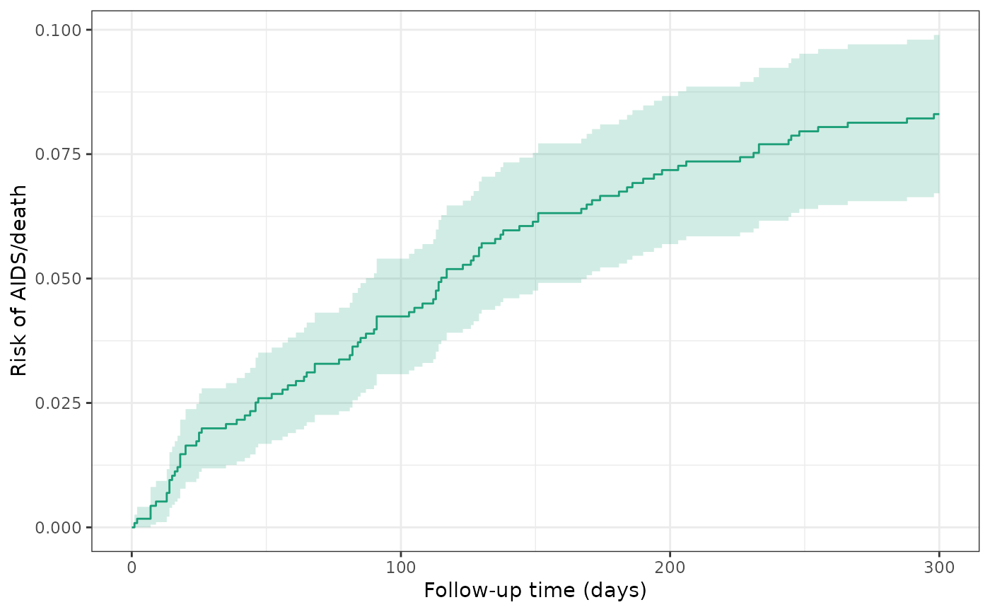
make_table2(actg_1, risk_time = 300)Model 2: Crude model of treatment and outcome
During the trial period, the cumulative incidence of AIDS or death was 10.9% among all dual therapy patients (untreated) and 5.7% for all triple therapy patients (treated). The crude RD for AIDS/death was -5.2%, indicating that treated patients had a lower risk of AIDS/death by approximately 5 percentage points.
ds_2 = specify_models(identify_treatment(art),
                    identify_outcome(y))

actg_2 = estimate_ipwrisk(actg, ds_2,
                     times=seq(0, 300, 1),
                     label = c("Unadjusted"))

plot(actg_2) +
  theme_bw() +
  xlab("Follow-up time (days)") +
  ylab("Risk of AIDS/death")
make_table2(actg_2, risk_time = 300)Model 3: Crude model of treatment and outcome, accounting for censoring
After censoring patients who dropped out during the trial period, the cumulative incidence of AIDS or death was 11.2% for dual therapy patients (untreated) and 5.8% for triple therapy patients (treated). The RD for AIDS/death was -5.3%, again indicating that treated patients had a lower risk of AIDS/death by approximately 5 percentage points.
ds_3 = specify_models(identify_treatment(art),
                    identify_censoring(drop_out),
                    identify_outcome(y))

actg_3 = estimate_ipwrisk(actg, ds_3,
                     times=seq(0, 300, 1),
                     label = c("Unadjusted, censor drop-out"))

plot(actg_3) +
  theme_bw() +
  xlab("Follow-up time (days)") +
  ylab("Risk of AIDS/death")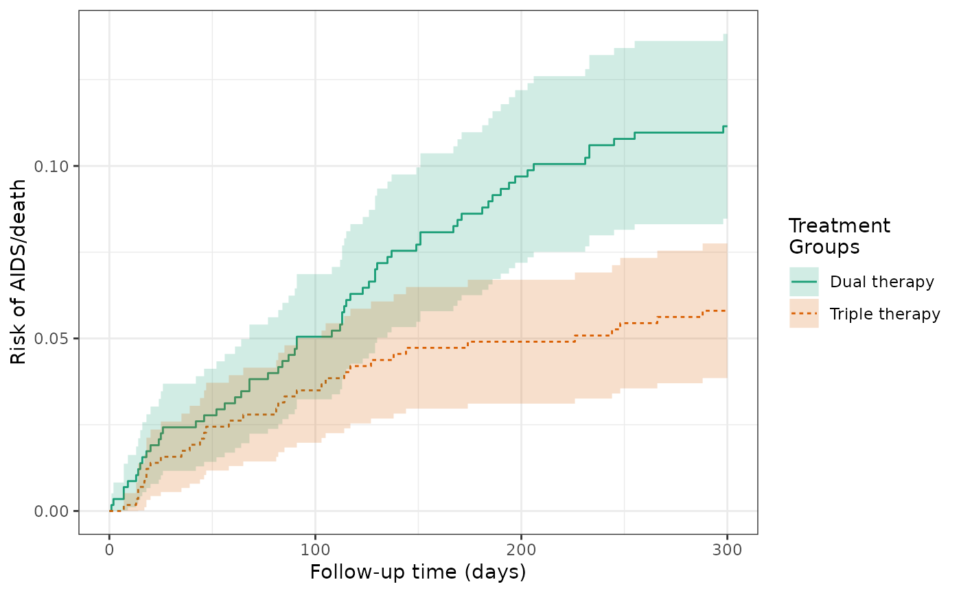
make_table2(actg_3, risk_time = 300)Model 4: IPTW model of treatment, G-computation estimator of risk, and augmented inverse probability weighted estimator
Although the treatment was randomized, chance imbalances between treatment gorups of CD4 cell count and other risk factors could exist. Adjustment for such factors could improve the efficiency of the estimator. Using the IPTW model, the cumulative incidence of AIDS or death was 10.9% for dual therapy patients (untreated) and 5.9% for triple therapy patients (treated). The weighted RD for AIDS/death was -5%, which is similar to the unweighted estimate.
ds_4 = specify_models(identify_treatment(art, formula = ~age + cd4 + sex + race + idu + karnofsky),
                    identify_censoring(drop_out),
                    identify_outcome(y))

actg_4 = estimate_ipwrisk(actg, ds_4,
                     times=seq(0, 300, 1),
                     label = c("IPTW"), nboot = 250)

plot(actg_4) +
  theme_bw() +
  xlab("Follow-up time (days)") +
  ylab("Risk of AIDS/death")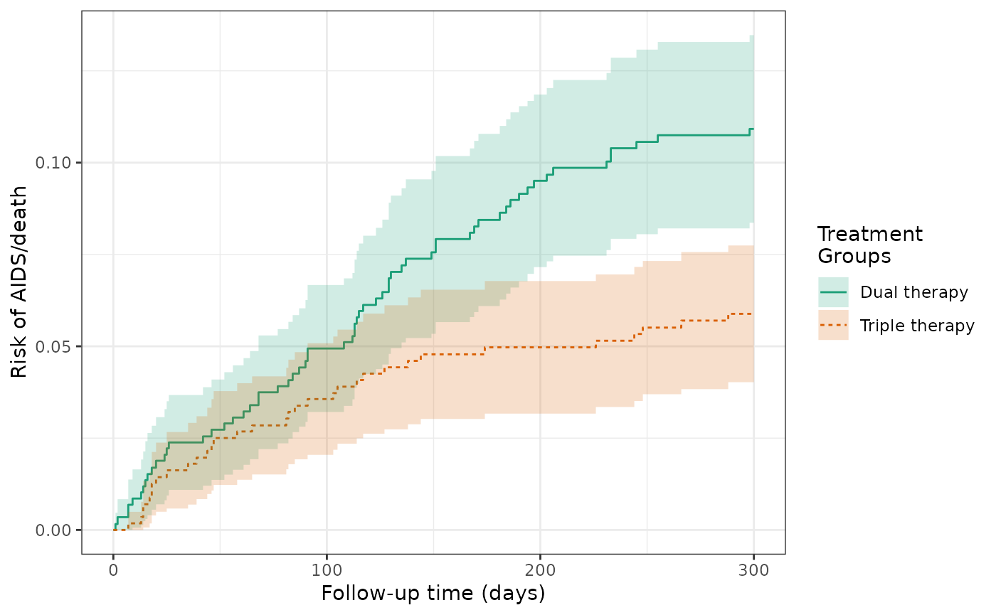
make_table2(actg_4, risk_time = 300)Given that the covariates were well balanced between treatment arms, the histogram shows a very limited distribution of propensity scores between the groups.
hist(actg_4) + theme_bw() + xlab("Propensity score")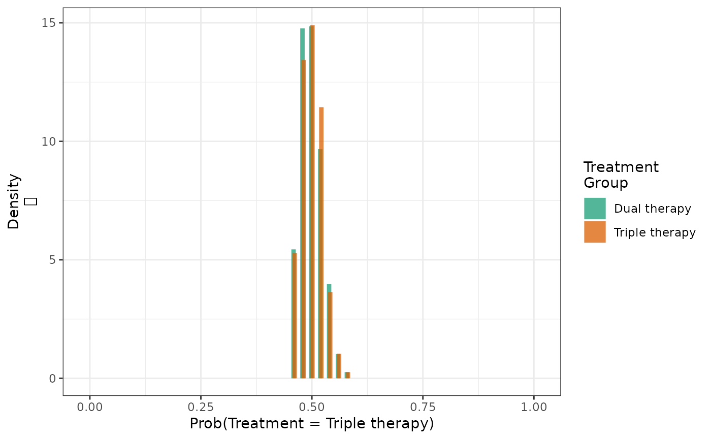
We can also estimate the cumulative risk using \(G\)-computation under an assumed Cox model.
ds_4g = specify_models(identify_treatment(art, formula = ~age +
                                            cd4 + sex + race + idu +
                                            karnofsky),
                    identify_censoring(drop_out),
                    identify_outcome(y, formula = ~age + cd4 + sex +
                                       race + idu + karnofsky))

actg_4g = estimate_gcomprisk(actg, ds_4g,
                     times=seq(0, 300, 1),
                     label = c("G-comp"), nboot = 250)

plot(actg_3, actg_4, actg_4g, rd = TRUE, overlay = TRUE) +
  theme_bw() +
  xlab("Follow-up time (days)") +
  ylab("Risk of AIDS/death")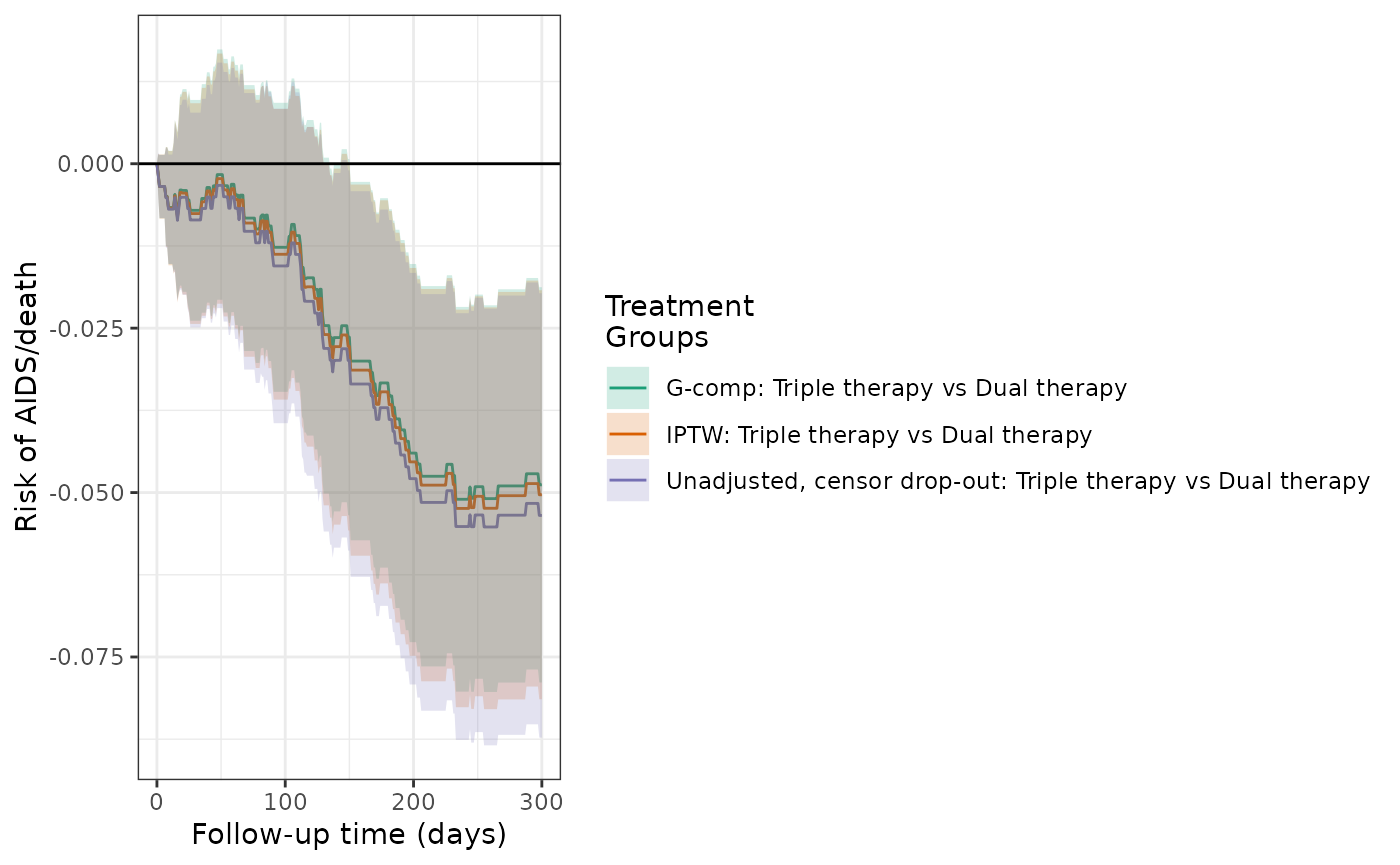
make_table2(actg_4, actg_4g, risk_time = 300)In the previous examples, each estimator required modeling the treatment and censoring processes (IPW) or the outcome process (G-computation). In these cases, if either model is misspecified, we do not expect the estimators to be consistent. To protect against model misspecification, augmented inverse probability weighted (AIPW) estimation utilizes all of the aforementioned models, and if either set is correctly specified, the resulting estimator is consistent. Additionally, the AIPW estimator is expected to be more efficient (narrower confidence intervals) than the IPW estimator, and non-conservative inference can be made without bootstrapping. The AIPW estimate of the RD was -5%, with marginally tighter confidence intervals than IPW.
actg_4aipw = estimate_aipwrisk(actg, ds_4g,
                     times=seq(0, 300, 1),
                     label = c("AIPW"))

plot(actg_3, actg_4, actg_4g, actg_4aipw, rd = TRUE, overlay = TRUE) +
  theme_bw() +
  xlab("Follow-up time (days)") +
  ylab("Risk of AIDS/death")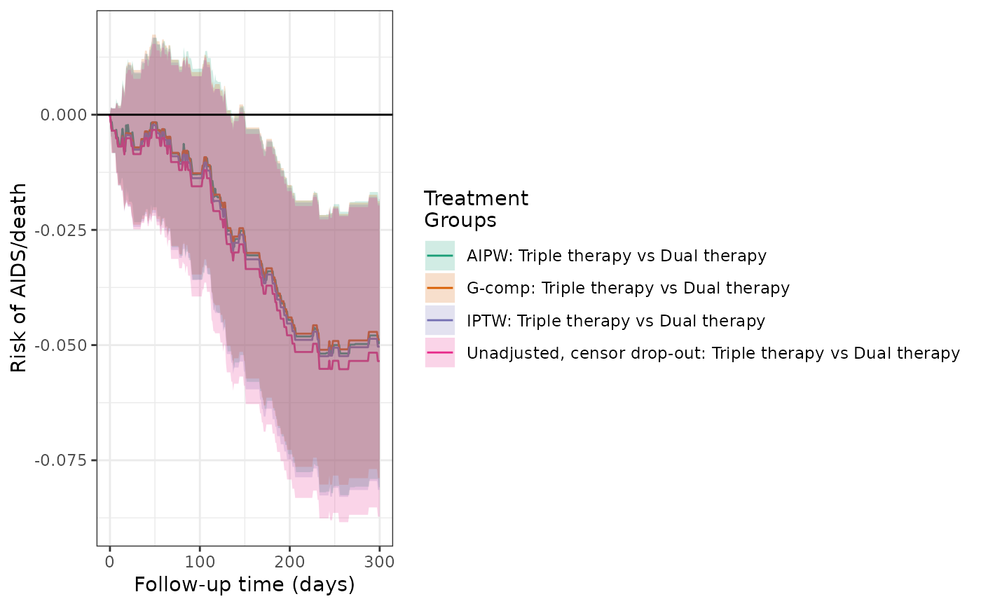
make_table2(actg_4, actg_4g, actg_4aipw, risk_time = 300)Models 5 and 6: IPTW models of hypothetical treatment and outcome, when confounding is induced
In the ACTG dataset, the variable ‘r’ is constructed to illustrate confounding and corresponds to patients who are in the subcohort (r=1). The distribution of CD4 count is not balanced between the two subcohort groups (where r=1 and r=0). The crude analysis indicates that participants in the subcohort (r=1) had a higher risk of treatment discontinuation, AIDS or death, and drop-out from the study. Overall, 74 participants in the subcohort experienced the outcome of AIDS or death, while 22 participants not in the subcohort experienced the outcome.
actg$r <- factor(actg$r, levels = c(0,1), labels = c("Not in subcohort","Subcohort"))

make_table1(actg, r, age, cd4, sex, race, idu, karnofsky)| Characteristic1 | Subcohort n=713 |
Not in subcohort n=443 |
|---|---|---|
| age, Mean (SD) | 39.16 (8.81) | 39.18 (8.72) |
| cd4, Mean (SD) | 75.81 (67.85) | 104.30 (69.93) |
| sex | ||
| Female | 118 16.55 | 82 18.51 |
| Male | 595 83.45 | 361 81.49 |
| race | ||
| White | 373 52.31 | 250 56.43 |
| Black | 128 17.95 | 77 17.38 |
| Hispanic | 212 29.73 | 116 26.19 |
| idu | ||
| No | 600 84.15 | 372 83.97 |
| Yes | 113 15.85 | 71 16.03 |
| karnofsky | ||
| Score < 90 | 132 18.51 | 82 18.51 |
| Score >= 90 | 581 81.49 | 361 81.49 |
| 1 All values are N (%) unless otherwise specified | ||
actg %>%
  group_by(r) %>%
  summarize(n=n(),
            `Number Stopping`=sum(!is.na(stop)),
            `Number w/ AIDS`=sum(!is.na(y)),
            `Number Dropping Out` = sum(!is.na(drop_out))) %>%
  mutate(`% Stop`=round(`Number Stopping`/n*100,1),
         `% AIDS`=round(`Number w/ AIDS`/n*100,1),
         `% Dropout`=round(`Number Dropping Out`/n*100,1))   %>%
kable()| r | n | Number Stopping | Number w/ AIDS | Number Dropping Out | % Stop | % AIDS | % Dropout |
|---|---|---|---|---|---|---|---|
| Not in subcohort | 443 | 43 | 22 | 14 | 9.7 | 5.0 | 3.2 |
| Subcohort | 713 | 174 | 74 | 37 | 24.4 | 10.4 | 5.2 |
Using the crude model of treatment (subcohort) and outcome, the cumulative incidence of AIDS or death was 10.6% for subcohort patients and 5.0% for patients not in the subcohort. The crude RD for AIDS/death was 5.6%, indicating that subcohort patients had a higher risk of AIDS/death by 5.6 percentage points.
ds_5 = specify_models(identify_treatment(r),
                    identify_censoring(drop_out),
                    identify_outcome(y))

actg_5 = estimate_ipwrisk(actg, ds_5,
                     times=seq(0, 300, 1),
                     label = c("Unadjusted, by subcohort"))

plot(actg_5) +
  theme_bw() +
  xlab("Follow-up time (days)") +
  ylab("Risk of AIDS/death")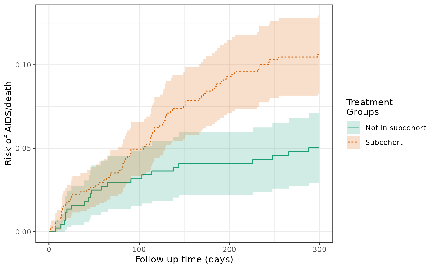
make_table2(actg_5, risk_time = 300)We then used an IPTW model to balance the subcohort groups on the baseline covariates and calculate a weighted RD. The cumulative incidence of AIDS or death was 9.7% for subcohort patients and 5.9% for patients not in the subcohort. The weighted RD for AIDS/death was 3.9%, which is attentuated compared to the unweighted estimate.
ds_6 = specify_models(
  identify_treatment(r, formula = ~age + cd4 + sex + race + idu + karnofsky),
  identify_censoring(drop_out),
  identify_outcome(y)
  )

actg_6 = estimate_ipwrisk(actg, ds_6,
                     times=seq(0, 300, 1),
                     label = c("IPTW, by subcohort"))

plot(actg_6) +
  theme_bw() +
  xlab("Follow-up time (days)") +
  ylab("Risk of AIDS/death")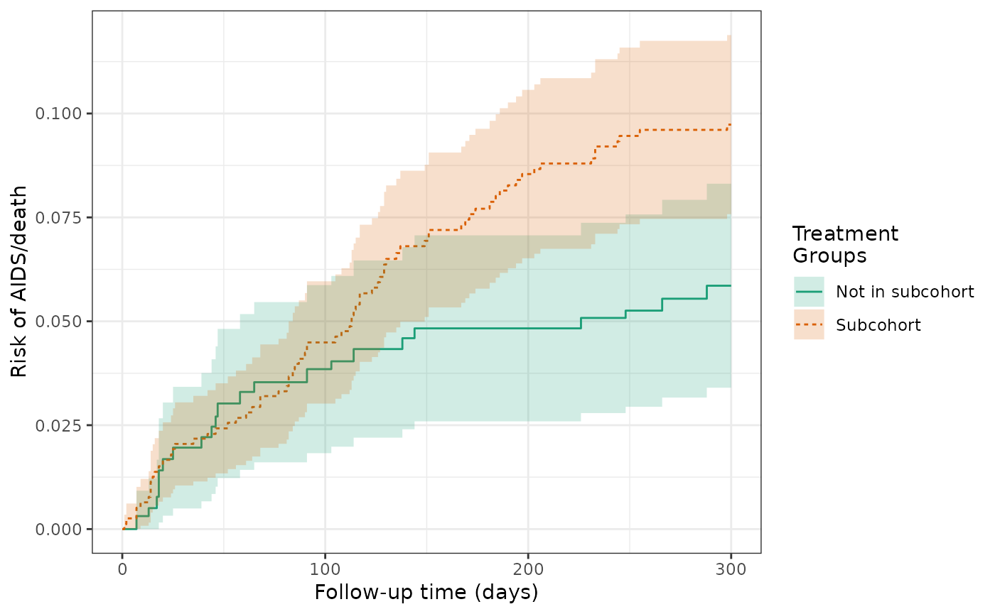
make_table2(actg_6, risk_time = 300)
plot(actg_5, actg_6, scales="fixed", overlay = TRUE)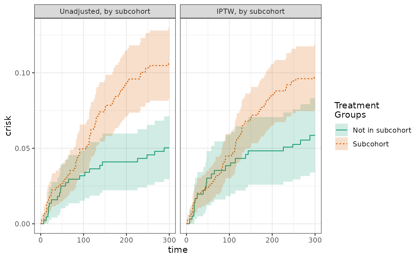
The histogram of the propensity score distribution shows that the assumption of positivity has not been violated.
hist(actg_6) + theme_bw() + xlab("Propensity score")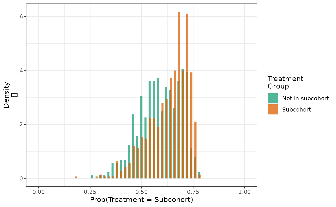
We can determine the extent to which weighting achieves balance of key confounders through computing the weighted means of baseline covariates by subcohort group.
make_table1(actg_6, age, cd4, sex, race, idu, karnofsky)| Characteristic1 | Subcohort n=1161.04 |
Not in subcohort n=1150.35 |
|---|---|---|
| age, Mean (SD) | 39.16 (8.87) | 39.17 (8.77) |
| cd4, Mean (SD) | 88.62 (75.69) | 88.23 (66.81) |
| sex | ||
| Female | 201 17.31 | 199 17.30 |
| Male | 960 82.68 | 951 82.67 |
| race | ||
| White | 628 54.09 | 620 53.90 |
| Black | 203 17.48 | 200 17.39 |
| Hispanic | 330 28.42 | 331 28.77 |
| idu | ||
| No | 973 83.80 | 966 83.97 |
| Yes | 188 16.19 | 184 16.00 |
| karnofsky | ||
| Score < 90 | 216 18.60 | 212 18.43 |
| Score >= 90 | 946 81.48 | 938 81.54 |
| 1 All values are N (%) unless otherwise specified | ||
Finally, we can summarize the distribution of weights by subcohort group to verify that there are no unusually large values.
make_wt_summary_table(actg_6)