Inverse Probability of Missingness Weighting

Data setup

This demonstration will use the example3 dataset included in the causalRisk package, which was generated using the coxed package. This dataset of 10,000 observations includes a treatment variable (Statin), an outcome variable (Death), a censoring variable (EndofEnrollment), and two covariates (X1 and X2). The data are setup such that X1 is a confounder and effect measure modifier and X2 is a predictor of the outcome, and censoring is non-informative.

Statin	X1	X2	EndofEnrollment	Death
Control	-0.5633082	0.2089505	NA	NA
Control	-0.3456137	1.7601274	NA	2.650168
Treat	0.3637345	-0.9931112	NA	NA
Control	0.0530444	-0.2091482	NA	19.365315
Control	0.2136881	-1.0809493	NA	60.591595
Control	0.5691088	0.3711670	NA	NA

Analysis without missing data

To begin, we conduct an analysis without missing data. The crude risk is 17.1% in the control group and 9.0% in the treated group. The adjusted risk is 15.2% in the control group and 9.8% in the treated group. The crude and adjusted risk differences are -8.1% and -5.4%, respectively.

  #No missingness, for comparisons
  models_nomiss_crude <- specify_models(identify_treatment(Statin),
                                        identify_censoring(EndofEnrollment),
                                        identify_outcome(Death))
  
  fit_nomiss_crude <- estimate_ipwrisk(data,
                                       models_nomiss_crude,
                                       times = seq(0,20,.1),
                                       labels = c("No missingness - Crude"))

  models_nomiss <- specify_models(identify_treatment(Statin, ~X1),
                                  identify_censoring(EndofEnrollment),
                                  identify_outcome(Death))
  
  fit_nomiss <- estimate_ipwrisk(data,
                                 models_nomiss,
                                 times = seq(0,20,.1),
                                 labels = c("No missingness"))
  
  plot(fit_nomiss_crude, fit_nomiss, ncol=2, scales="fixed")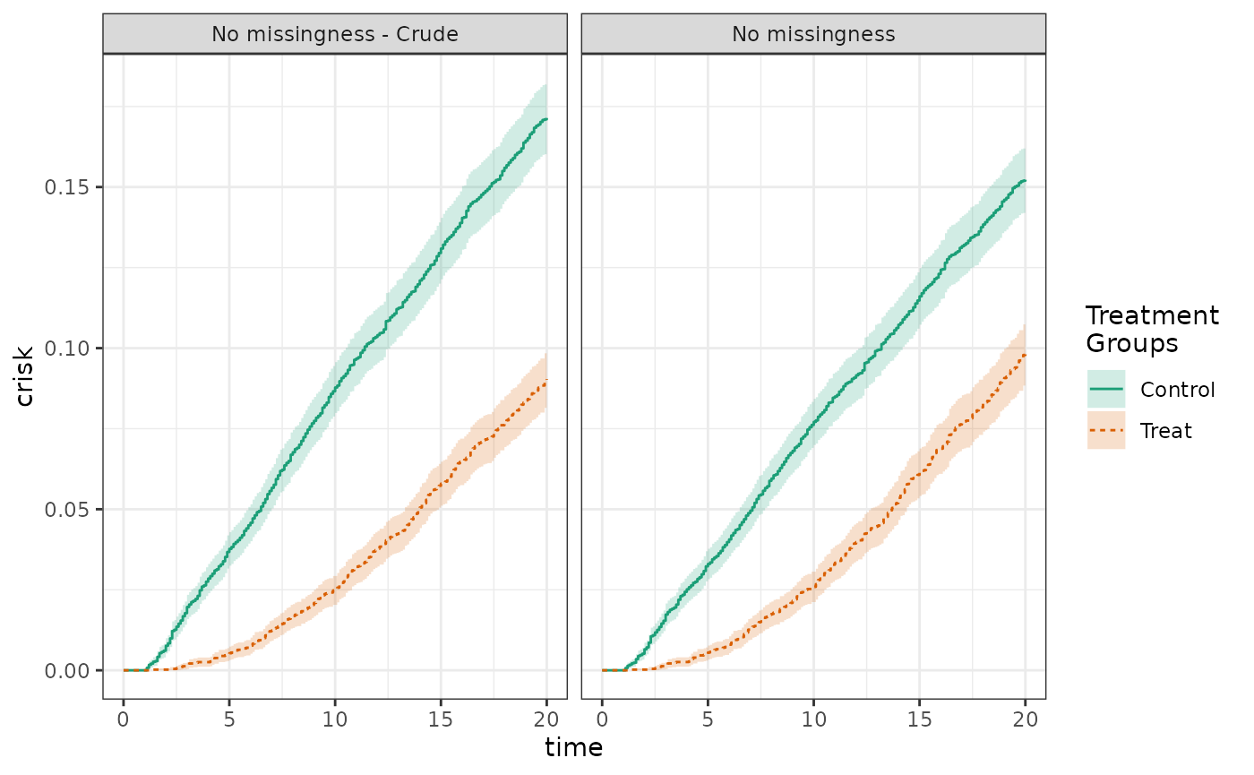

  make_table2(fit_nomiss_crude, fit_nomiss, risk_time=20)

Analysis with data missing completely at random (MCAR)

Next, we induce missingness that is MCAR, meaning that missingness is unconditionally independent of the outcome. We compare adjusted analyses of the full data, of the complete cases, and using inverse probability of missingness weights. Because the data are MCAR and the missingness model does not contain covariates, the complete case and IPMW analyses are essentially the same. In each analysis, the adjusted risk in the control group is 15.2%, in the treated is 10.1%, yielding a risk difference of -5.2%.

#Induce MCAR
data_mcar <- data
pmiss <- .10
miss <- rbinom(nrow(data_mcar),1,pmiss)
data_mcar$X1 <- ifelse(miss, NA, data_mcar$X1)

#Analyze
models_mcar <- specify_models(identify_treatment(Statin, ~X1),
                              identify_censoring(EndofEnrollment),
                              identify_outcome(Death),
                              identify_missing(~1))

fit_mcar <- estimate_ipwrisk(data_mcar,
                             models_mcar,
                             times = seq(0,20,.1),
                             labels = c("IPMW - MCAR"))

models_mcar_cc <- specify_models(identify_treatment(Statin, ~X1),
                                 identify_censoring(EndofEnrollment),
                                 identify_outcome(Death))

fit_mcar_cc <- estimate_ipwrisk(data_mcar,
                                models_mcar_cc,
                                times = seq(0,20,.1),
                                labels = c("Complete case - MCAR"))

plot(fit_nomiss, fit_mcar_cc, fit_mcar, ncol=3, scales="fixed")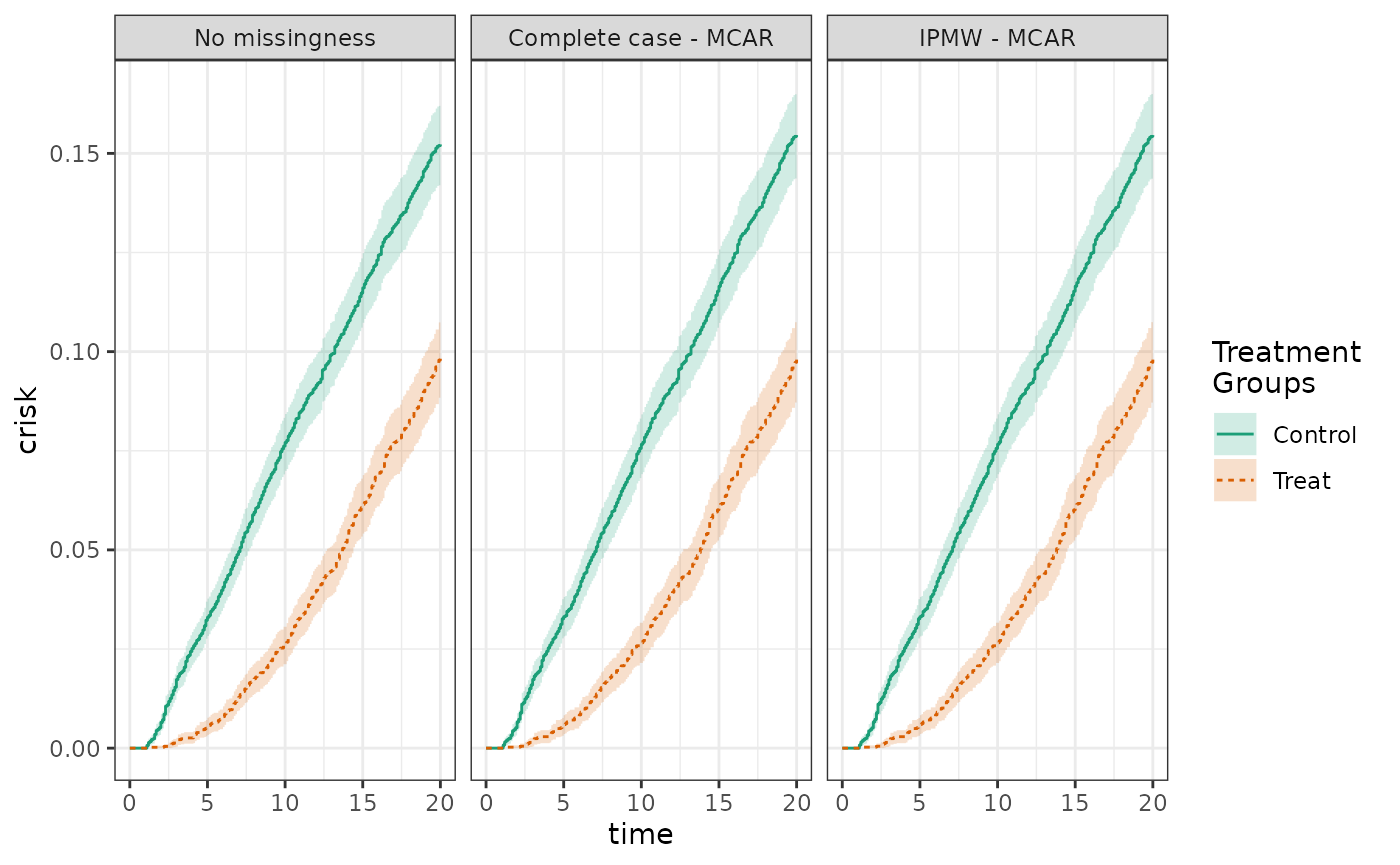

make_table2(fit_nomiss, fit_mcar_cc, fit_mcar, risk_time=20)

Analysis with data missing at random (MAR)

Finally, we induce missingness that is MAR, meaning that missingness is independent of the outcome conditional on some variables, in this case X2. Again, we compare adjusted analyses of the full data, of the complete cases, and using inverse probability of missingness weights. Because of the missing data structure, we expect the estimates from the complete case analysis to be biased, but for the IPMW to be unbiased. Indeed, the risks from the complete case analysis are 12.3% and 7.6% for the control and treatment groups, respectively, yielding a risk difference of -4.7%. The risks from the IPMW analysis are 15.3% and 9.1% for the control and treatment groups, respectively, for a risk difference of -6.2%.

#Induce MAR
data_mar <- data
data_mar$pmiss <- 1/(1+exp(-(log(.9)+log(5)*data_mar$X2)))
data_mar$miss <- apply(as.data.frame(data_mar$pmiss), 1, function(df) rbinom(1,1,df))
data_mar$X1 <- ifelse(data_mar$miss==1, NA, data_mar$X1)

#Analyze
models_mar <- specify_models(identify_treatment(Statin, ~X1),
                             identify_censoring(EndofEnrollment),
                             identify_outcome(Death),
                             identify_missing(~X2))

fit_mar <- estimate_ipwrisk(data_mar,
                            models_mar,
                            times = seq(0,20,.1),
                            labels = c("IPMW - MAR"))

models_mar_cc <- specify_models(identify_treatment(Statin, ~X1),
                                identify_censoring(EndofEnrollment),
                                identify_outcome(Death))

fit_mar_cc <- estimate_ipwrisk(data_mar,
                               models_mar_cc,
                               times = seq(0,20,.1),
                               labels = c("Complete case - MAR"))

plot(fit_nomiss, fit_mar_cc, fit_mar, scales="fixed", ncol=3)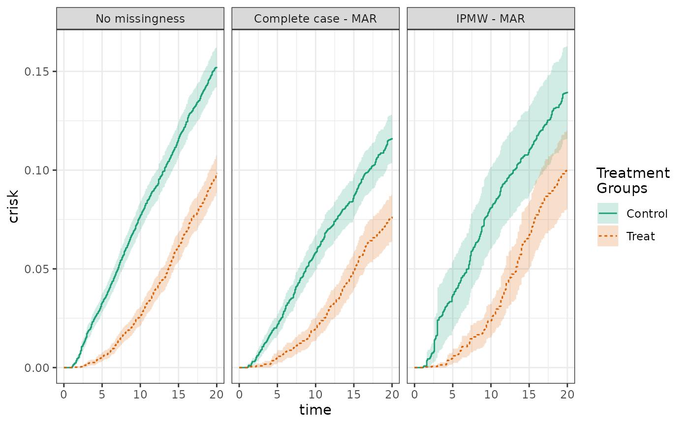

make_table2(fit_nomiss, fit_mar_cc, fit_mar, risk_time=20)