Re-analysis of the WIHS 2009 cohort with causalRisk
wihs.RmdIntroduction
The WIHS 2009 dataset consists of 1,164 women enrolled in WIHS who were HIV-positive, free of clinical AIDS, and not on antiretroviral therapy (ART) at study baseline (Dec. 6, 1995). These data were used in Lau, Cole, and Gange’s 2009 paper in the American Journal of Epidemiology on using competing risk regression models with epidemiologic data. Women were followed until initiation of antiretroviral therapy (ART), AIDS diagnosis, death, or administrative censoring. Administrative censoring took place at 10 years in our WIHS package data, which differs slightly from the administrative censoring date of Sept. 28, 2006 in the Lau paper (which resulted in 10.8 years of follow-up).
The outcomes of interest in the data are ART initiation, AIDS, and death. The main exposure is history of injection drug use. At start of follow-up, 439 women (38%) reported a history of injection drug use, and 725 women (62%) had no history of injection drug use. There were imbalances in the distribution of covariates (race, age, and CD4 cell count at baseline) by exposure. Participants with a history of injection drug use were more likely to be older and African American. Participants had similar CD4 cell counts across exposure levels.
make_table1(wihs, idu, white, age, cd4, tab_stat = "Median",
tab_stat2 = "IQR", smd = T, graph = T)| Characteristic1 | History of IDU n=439 |
No IDU n=725 |
SMD | Graph |
|---|---|---|---|---|
| white | 0.145599962088702 |  |
||
| Non-white Race | 273 62.19 | 399 55.03 |  |
|
| White Race | 166 37.81 | 326 44.97 | |
|
| age, Median (IQR) | 40.00 (35.00, 44.00) | 33.00 (29.00, 39.00) | -0.705925229577615 |  |
| cd4, Median (IQR) | 352.00 (208.50, 522.00) | 348.00 (216.00, 505.00) | -0.0651706794527488 |  |
| 1 All values are N (%) unless otherwise specified | ||||
ART initiation and AIDS diagnosis or death are competing outcomes in the study. The crude analysis by exposure shows the 10-year risk of ART initiation is higher for participants without a history of injection drug use. The WIHS dataset used by Lau was not censored at 10 years (study continued for an additional ~9 months), so has 8 additional women initiating ART (who did so when t>10): 679 total (469 no IDU, 210 IDU) in Lau vs. 671 total (463 no IDU, 208 IDU) in our data.
wihs %>%
  group_by(idu) %>%
  dplyr::summarize(n=n(),`Number on  ART` = sum(!is.na(art)),
                   `Risk of initiatig ART`=round(sum(!is.na(art))/n(),2)) %>%
kable()| idu | n | Number on ART | Risk of initiatig ART |
|---|---|---|---|
| No IDU | 725 | 463 | 0.64 |
| History of IDU | 439 | 208 | 0.47 |
The crude analysis by exposure shows that the 10-year risk of AIDS or death (prior to ART initiation) is higher for participants with a history of injection drug use. The WIHS dataset used by Lau has 3 additional women who experienced the outcomes of AIDS diagnosis or death (which occurred when t>10): 359 total (169 no IDU, 190 IDU) in the Lau paper vs. 356 total (168 no IDU, 188 IDU) in our data.
wihs %>%
  group_by(idu) %>%
  dplyr::summarize(n=n(),
          `Number of AIDS or Death` = sum(!is.na(aids_death_art))-sum(j,na.rm = T),
          `Risk of AIDS or Death` =
            round((sum(!is.na(aids_death_art))-sum(j,na.rm = T))/n(),2)) %>%
kable()| idu | n | Number of AIDS or Death | Risk of AIDS or Death |
|---|---|---|---|
| No IDU | 725 | 168 | 0.23 |
| History of IDU | 439 | 188 | 0.43 |
Among the 1,164 women enrolled in WIHS, there were 223 who initiated ART and later received an AIDS diagnosis or died (experienced both outcomes). 137 women did not experience either outcome.
Cumulative risks of the competing outcomes (ART initiation, AIDS/death) among all participants
Over ten years, the cumulative risk of ART initiation among WIHS participants is 57.6% (671 events/1164 total sample size).
ds_art = specify_models(identify_outcome(art))

wihs_art = estimate_ipwrisk(wihs, ds_art, times = seq(0,10,0.01),
                       label = c("wihs ART overall risk"))
plot(wihs_art) +
  xlab("Follow-up time (years)") +
  ylab("Risk of ART initiation") +
  ylim(0,1)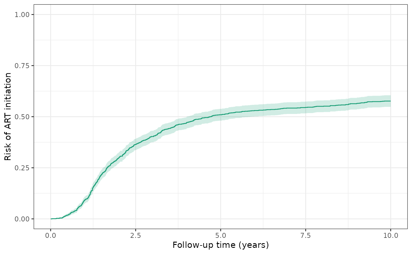
make_table2(wihs_art, risk_time = 10)Over ten years, the cumulative risk of AIDS or death among WIHS participants is 49.7% (579 events / 1164 patients), regardless of ART initiation.
ds_aids = specify_models(identify_outcome(aids_death))

wihs_aids = estimate_ipwrisk(wihs, ds_aids,
                        times = seq(0,10,0.01),
                        label = c("wihs AIDS overall risk"))

plot(wihs_aids) +
  xlab("Follow-up time (years)") +
  ylab("Risk of AIDS or death") +
  ylim(0,1)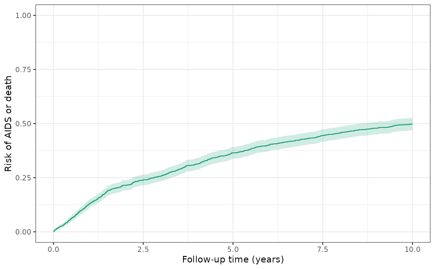
make_table2(wihs_aids, risk_time = 10)Model 1: Crude model of exposure and cause-specific cumulative incidence
Over ten years, the cause-specific cumulative incidence of ART initiation is 85.8% for the unexposed (no history of IDU) and is 77.3% for the exposed (history of IDU). This is similar to Figure 3A in the Lau paper; these estimates of cause-specific incidence are slightly lower than those in Figure 3A due to the discrepancies in sample size (WIHS dataset used by Lau was not censored at 10 years and has 8 additional women initiating ART). Here, the cause-specific crude RD for ART initiation is -8.5%, corresponding to a lower risk of ART initiation among the exposed.
ds1_art = specify_models(identify_treatment(idu),
                       identify_censoring(aids_death),
                       identify_censoring(dropout),
                       identify_outcome(art))

wihs1_art = estimate_ipwrisk(wihs, ds1_art,
                        times = seq(0,10,0.01),
                        label = c("wihs1 ART cause-specific incidence"))
plot(wihs1_art) +
  xlab("Follow-up time (years)") +
  ylab("Risk of ART initiation") +
  ylim(0,1)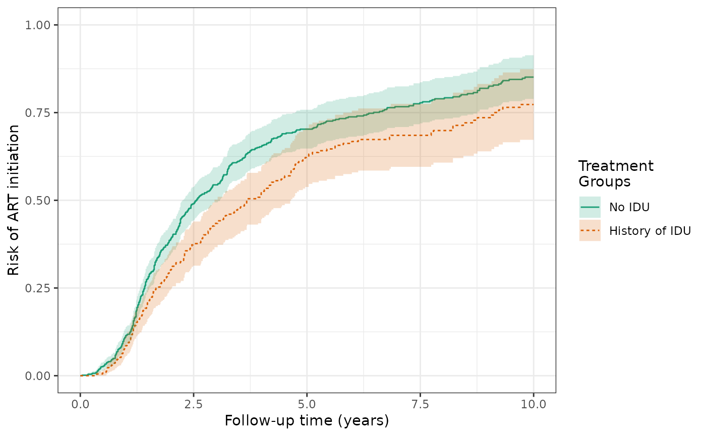
make_table2(wihs1_art, risk_time = 10)Over ten years, the cause-specific cumulative incidence of AIDS/death is 44.2% for the unexposed and is 67.7% for the exposed. This is similar to Figure 3C in the Lau paper. Again, these estimates of cause-specific incidence are slightly lower than those in Figure 3C due to the discrepancies in sample size (WIHS dataset used by Lau was not censored at 10 years and has 3 additional women who experienced the outcomes of AIDS diagnosis or death). The cause-specific crude RD for AIDS/death is 23.6%, corresponding to a higher risk of AIDS/death among the exposed.
ds1_aids = specify_models(identify_treatment(idu),
                      identify_censoring(art),
                      identify_censoring(dropout),
                      identify_outcome(aids_death))

wihs1_aids = estimate_ipwrisk(wihs, ds1_aids,
                         times = seq(0,10,0.01),
                         label = c("wihs1 AIDS cause-specific incidence"))
plot(wihs1_aids) +
  xlab("Follow-up time (years)") +
  ylab("Risk of AIDS or death") +
  ylim(0,1)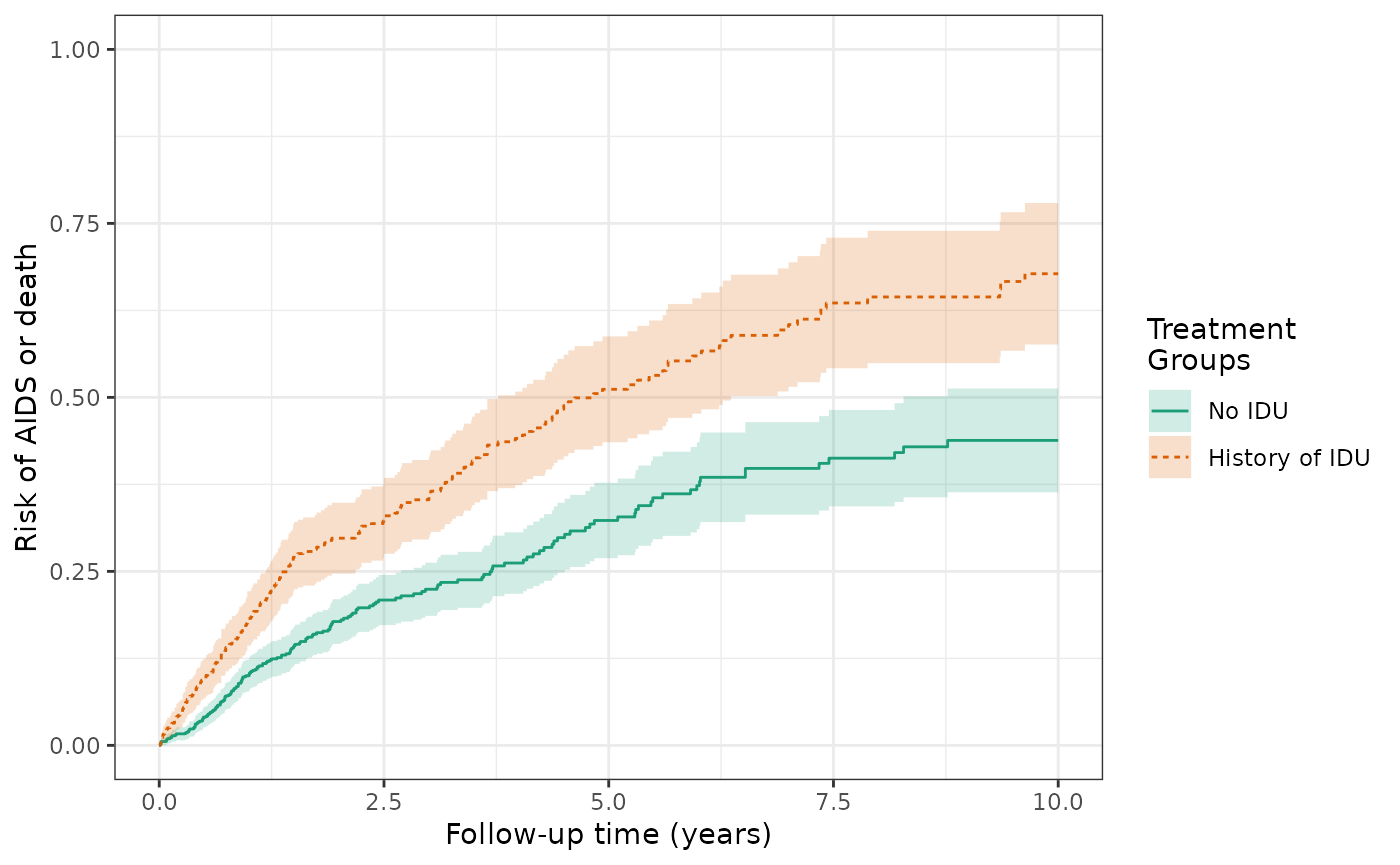
make_table2(wihs1_aids, risk_time = 10)Model 2: Crude models of exposure and cumulative incidence of outcome
The crude risks of the ART initiation outcome at 10 years are 48.4% for the exposed (history of IDU) and 66.8% for the unexposed (no IDU), making the crude RD = -18.5%. This is similar to Figure 3B in the Lau paper (but no weights applied yet).
ds2_art = specify_models(identify_treatment(idu),
                      identify_censoring(dropout),
                      identify_outcome(art))

wihs2_art = estimate_ipwrisk(wihs, ds2_art,
                        times = seq(0,10,0.01),
                        label = c("wihs2 ART crude model"))
plot(wihs2_art) +
  xlab("Follow-up time (years)") +
  ylab("Risk of ART initiation") +
  ylim(0,1)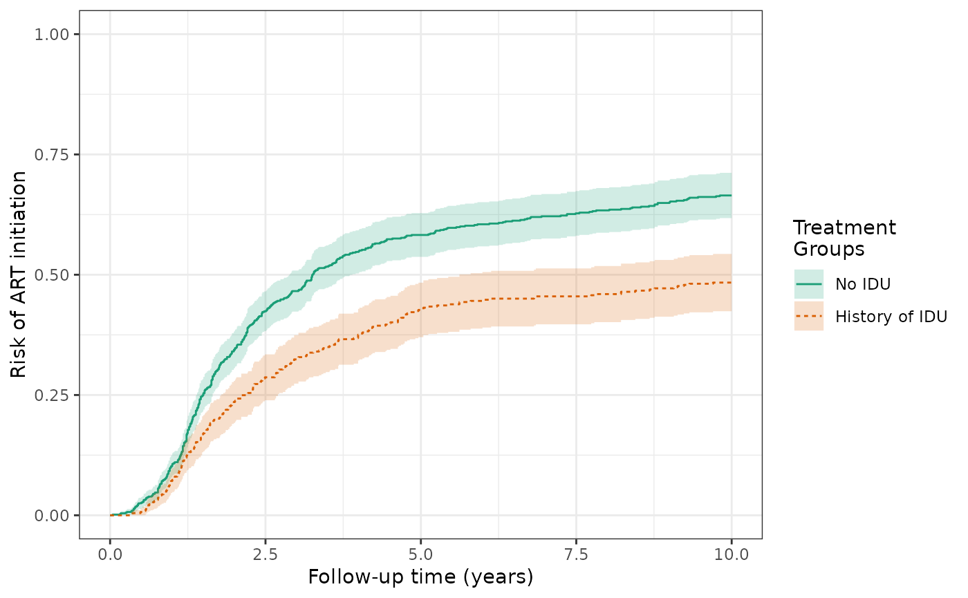
make_table2(wihs2_art, risk_time = 10)The crude risks of the AIDS/death outcome at 10 years are 43.8% for the exposed and 24.1% for the unexposed, making the crude RD = 19.7%. This is similar to Figure 3D in the Lau paper (again, no weights applied yet).
wihs$aids_death_before_art =
  ifelse(!is.na(wihs$aids_death_art) & wihs$j==0, wihs$aids_death, NA)

ds2_aids = specify_models(identify_treatment(idu),
                        identify_censoring(dropout),
                        identify_outcome(aids_death_before_art))

wihs2_aids = estimate_ipwrisk(wihs, ds2_aids,
                         times = seq(0,10,0.01),
                         label = c("wihs2 AIDS crude model"))

plot(wihs2_aids) +
  xlab("Follow-up time (years)") +
  ylab("Risk of AIDS or death") +
  ylim(0,1)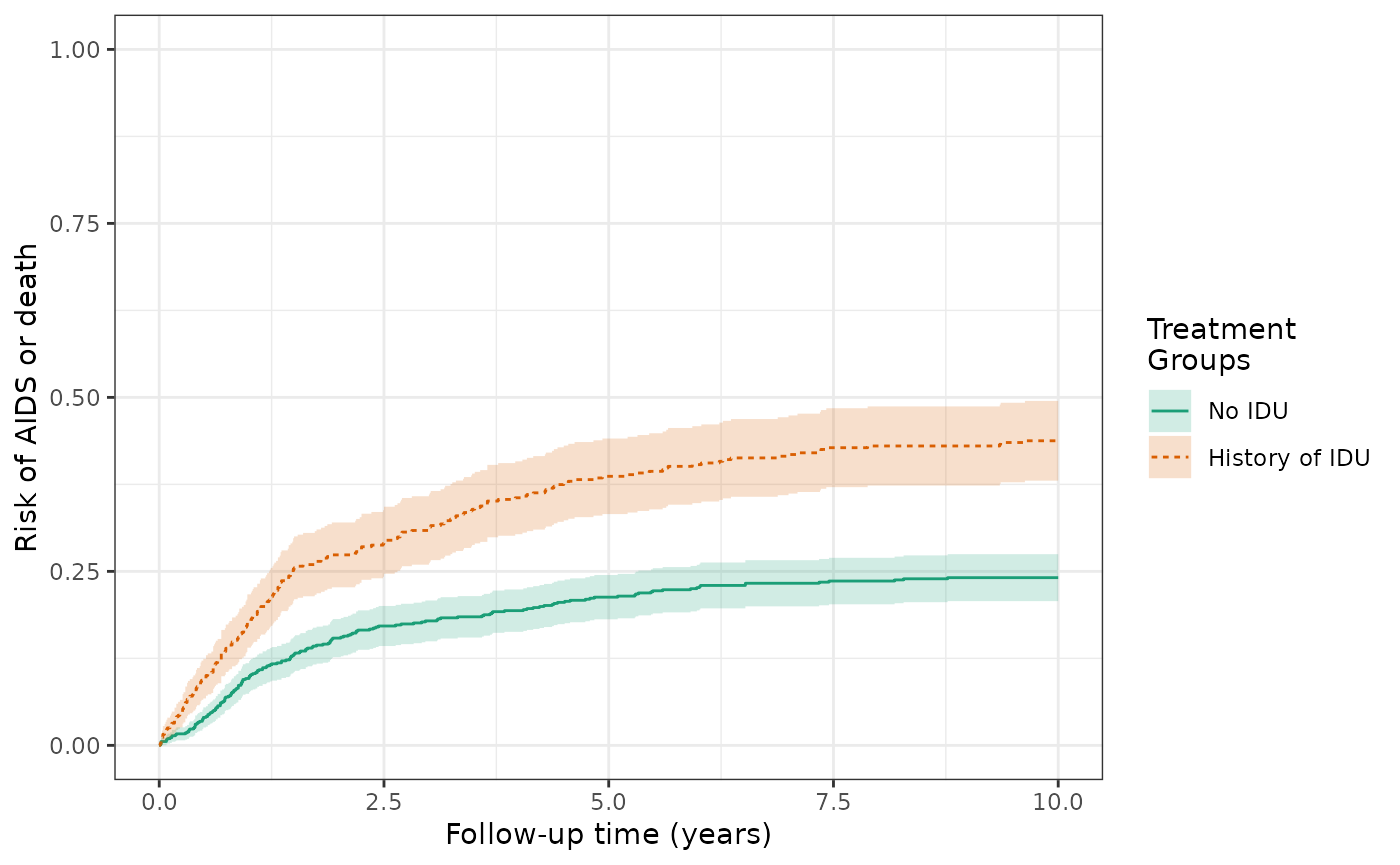
make_table2(wihs2_aids, risk_time = 10)Model 3: Inverse-probability of treatment weighted (IPTW) model for exposure and outcome
The IP-weighted risk of the ART outcome at 10 years are 46.6% for the exposed and 71.7% for the unexposed, and the cumulative risk difference increases in magnitude from -18.5% (crude) to -25.1% (IPTW). The plot of IP-weighted risk by exposure is similar to Figure 3B in the Lau paper (slightly different estimator used).
ds3_art = specify_models(identify_treatment(idu, formula = ~white + age + cd4),
                       identify_censoring(dropout),
                       identify_outcome(art))

wihs3_art = estimate_ipwrisk(wihs, ds3_art,
                        times = seq(0,10,0.01),
                        label = c("wihs3 ART IPTW model"))

plot(wihs3_art) +
  xlab("Follow-up time (years)") +
  ylab("Risk of ART initiation") +
  ylim(0,1)
make_table2(wihs3_art, risk_time = 10)The IP-weighted risks of the AIDS/death outcome (prior to ART initiation) at 10 years are 41.0% for the exposed and 24.5% for the unexposed, and the cumulative risk difference attentuates from 19.7% (crude) to 16.5% (IPTW). This is similar to Figure 3D in the Lau paper (slightly different estimator used).
ds3_aids = specify_models(identify_treatment(idu, formula = ~white + age + cd4),
                        identify_censoring(dropout),
                        identify_outcome(aids_death_before_art))

wihs3_aids = estimate_ipwrisk(wihs, ds3_aids,
                         times = seq(0,10,0.01),
                         label = c("wihs3 AIDS IPTW model"))
plot(wihs3_aids) +
  xlab("Follow-up time (years)") +
  ylab("Risk of AIDS or death") +
  ylim(0,1)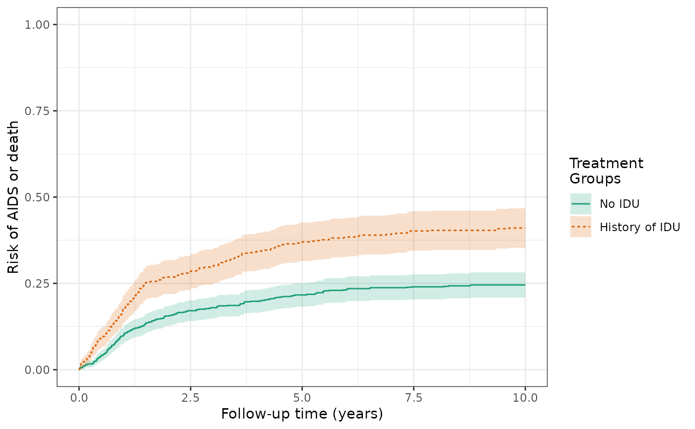
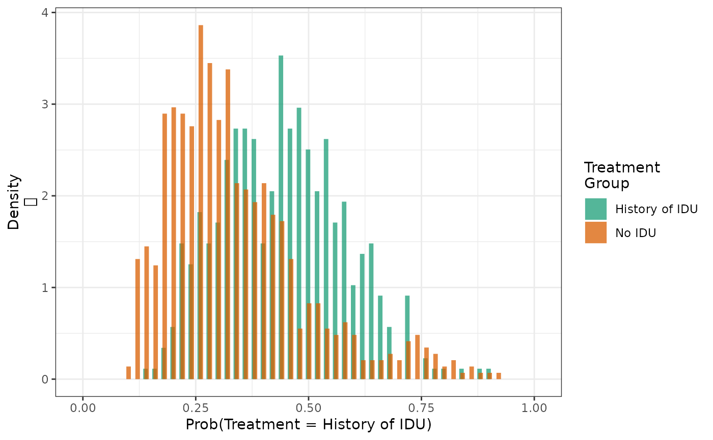
make_table2(wihs3_aids, risk_time = 10)The histogram of the propensity score distribution shows that the assumption of positivity has not been violated.
We can determine the extent to which weighting achieves balance of key confounders through computing the weighted means of baseline covariates by exposure group.
make_table1(wihs3_art, white, age, cd4, smd = T)| Characteristic1 | History of IDU n=1103.26 |
No IDU n=1222.53 |
SMD |
|---|---|---|---|
| white | 0.0172731787491934 | ||
| Non-white Race | 613 55.56 | 690 56.44 | |
| White Race | 490 44.41 | 533 43.60 | |
| age, Mean (SD) | 37.72 (6.31) | 38.15 (11.07) | 0.057653767040622 |
| cd4, Mean (SD) | 389.12 (261.87) | 387.63 (260.88) | -0.00559315968845884 |
| 1 All values are N (%) unless otherwise specified | |||
Finally, we can summarize the distribution of weights by exposure group to verify that there are no unusually large values. The sum of the standard weight should be approximately equal to \(n\) in each group.
make_wt_summary_table(wihs3_art)Although the variables seem fairly well balanced, to improve balance of confounders that may be somewhat out of balance, we can create interactions with the offending variables or, if the variable is continuous, have the varible enter the model thorugh a spline term. We do this below with age:
ds3_aids_sens = specify_models(
  identify_treatment(idu, formula = ~white + bs(age) + cd4),
  identify_censoring(dropout),
  identify_outcome(aids_death_before_art))

wihs3_aids_sens = estimate_ipwrisk(wihs, ds3_aids_sens,
                         times = seq(0,10,0.01),
                         label = c("wihs3 AIDS IPTW model"))

make_table1(wihs3_aids_sens, white, age, cd4, smd = T)| Characteristic1 | History of IDU n=1200.97 |
No IDU n=1155.93 |
SMD |
|---|---|---|---|
| white | 0.044044630758909 | ||
| Non-white Race | 654 54.46 | 654 56.58 | |
| White Race | 547 45.55 | 502 43.43 | |
| age, Mean (SD) | 36.54 (8.78) | 36.38 (8.21) | -0.0209683598515796 |
| cd4, Mean (SD) | 402.87 (268.20) | 393.23 (266.99) | -0.0362207514259797 |
| 1 All values are N (%) unless otherwise specified | |||
In the resulting table 1, we see moderately improved balance of age across treatment arms.
Model 4: Inverse-probability of treatment and censoring weighted (IPTW+IPCW) model for exposure and outcome
The IP-weighted risk of the ART outcome at 10 years are 46.7% for the exposed and 71.5% for the unexposed, and the cumulative risk difference decreases in magnitude from -25.1% (IPTW) to -24.8% (IPTW+ICPW).
ds4_art = specify_models(identify_treatment(idu, formula = ~white+age+cd4),
                           identify_censoring(dropout, formula = ~white+age+cd4),
                           identify_outcome(art))

wihs4_art = estimate_ipwrisk(wihs, ds4_art,
                        times = seq(0,10,0.01),
                        label = c("wihs4 ART IPTW + IPCW model"))
plot(wihs4_art) +
  xlab("Follow-up time (years)") +
  ylab("Risk of ART initiation") +
  ylim(0,1)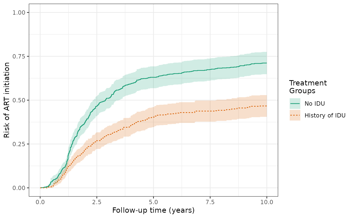
make_table2(wihs4_art, risk_time = 10)The IP-weighted risks of the AIDS/death outcome (prior to ART initiation) at 10 years are 41.1% for the exposed and 24.6% for the unexposed, and the cumulative risk difference remains 16.5% (IPTW and IPTW+IPCW).
ds4_aids =
  specify_models(identify_treatment(idu, formula = ~white + age + cd4),
                 identify_censoring(dropout, formula = ~white + age + cd4),
                 identify_outcome(aids_death_before_art))

wihs4_aids = estimate_ipwrisk(wihs, ds4_aids,
                         times = seq(0,10,0.01),
                         label = c("wihs4 AIDS IPTW + IPCW model"))
plot(wihs4_aids) +
  xlab("Follow-up time (years)") +
  ylab("Risk of AIDS or death") +
  ylim(0,1)
make_table2(wihs4_aids, risk_time = 10)Computing the weighted means of baseline covariates produces the same results as the IPTW model. The distribution of weights by exposure group is also the same.
make_table1(wihs4_art, white, age, cd4)| Characteristic1 | History of IDU n=1103.26 |
No IDU n=1222.53 |
|---|---|---|
| white | ||
| Non-white Race | 613 55.56 | 690 56.44 |
| White Race | 490 44.41 | 533 43.60 |
| age, Mean (SD) | 37.72 (6.31) | 38.15 (11.07) |
| cd4, Mean (SD) | 389.12 (261.87) | 387.63 (260.88) |
| 1 All values are N (%) unless otherwise specified | ||
make_wt_summary_table(wihs4_art)Model 5: Augmented inverse probability weighted estimation
The validity of the IP-weighted risk relies on correct specification of the models for censoring and treatment. If either of these models are misspecified, we do not expect the IP-weighted estimator to be consistent. To aid in protecting against model misspecification, augmented inverse probability weighted (AIPW) estimators additionally use a model for the outcome. If the outcome model or the censoring and treatment models are correctly specified, the estimator remains consistent. Additionally, if both models are correctly specified, we expect the AIPW estimator to be more efficient. The AIPW estimated risks of the ART outcome differ substantially from the IPTW+IPCW estimates, with estimates of 66.9% for the unexposed and 48.9% for the exposed, yielding a risk difference of 18.0% and substantially narrower confidence limits. The difference in the results suggests that the models used for IPTW+IPCW may be misspecified.
ds4_art_aipw = specify_models(identify_treatment(idu, formula = ~white+age+cd4),
                           identify_censoring(dropout, formula = ~white+age+cd4),
                           identify_outcome(art, formula = ~white+age+cd4))

wihs4_art_aipw = estimate_aipwrisk(wihs, ds4_art_aipw,
                        times = seq(0,10,0.01),
                        label = c("wihs4 ART AIPW model"))
plot(wihs4_art_aipw) +
  xlab("Follow-up time (years)") +
  ylab("Risk of ART initiation") +
  ylim(0,1)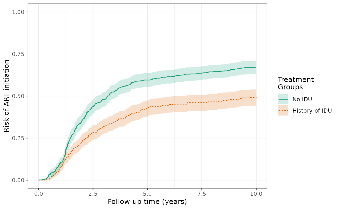
make_table2(wihs4_art, wihs4_art_aipw, risk_time = 10)We also see differences for the AIDS/death outcome. The AIPW risks of the AIDS/death outcome (prior to ART initiation) at 10 years are 43.0% for the exposed and 22.6% for the unexposed, and the cumulative risk difference is 20.3%.
ds4_aids_aipw =
  specify_models(identify_treatment(idu, formula = ~white + age + cd4),
                 identify_censoring(dropout, formula = ~white + age + cd4),
                 identify_outcome(aids_death_before_art, formula= ~white + age + cd4))

wihs4_aids_aipw = estimate_aipwrisk(wihs, ds4_aids_aipw,
                         times = seq(0,10,0.01),
                         label = c("wihs4 AIDS AIPW"))
plot(wihs4_aids_aipw) +
  xlab("Follow-up time (years)") +
  ylab("Risk of AIDS or death") +
  ylim(0,1)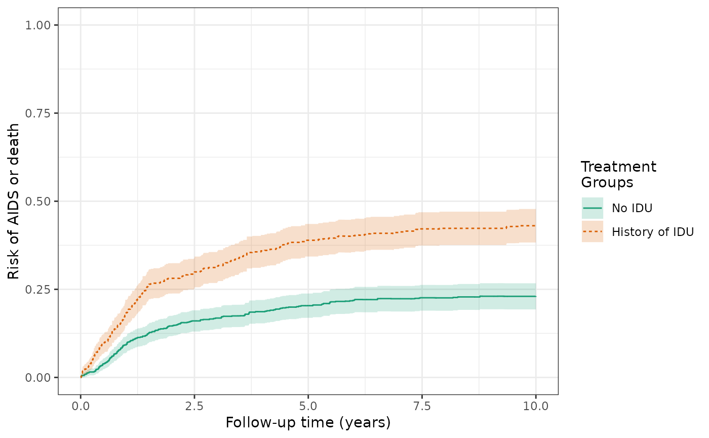
make_table2(wihs4_aids, wihs4_aids_aipw, risk_time = 10)Model 6: Standardized mortality ratio (SMR) weighted model for exposure and outcome
An alternative weighting scheme is to use SMR weights to estimate the effect of the IDU exposure on the outcomes of ART initiation and AIDS/death. Using SMR weights estimates an effect that generalizes to a particular subgroup of the population. In this case, we are interested in preventing the exposure of injection drug use among those participants who were exposed (i.e., had a history of injection drug use).
The SMR-weighted risk of the ART outcome at 10 years are 49.9% for the exposed and 66.9% for the unexposed, with a cumulative risk difference of -17%. This risk difference represents the effect of the exposure among the exposed and is decreased in magnitude from the IP weighted RD of -25%, which was standardized to the total population (rather than just the exposed).
wihs4_art_smr = estimate_ipwrisk(wihs, ds4_art,
                        times = seq(0,10,0.01),
                        wt_type = 1,
                        label = c("wihs4 ART SMR model"))
plot(wihs4_art_smr) +
  xlab("Follow-up time (years)") +
  ylab("Risk of ART initiation") +
  ylim(0,1)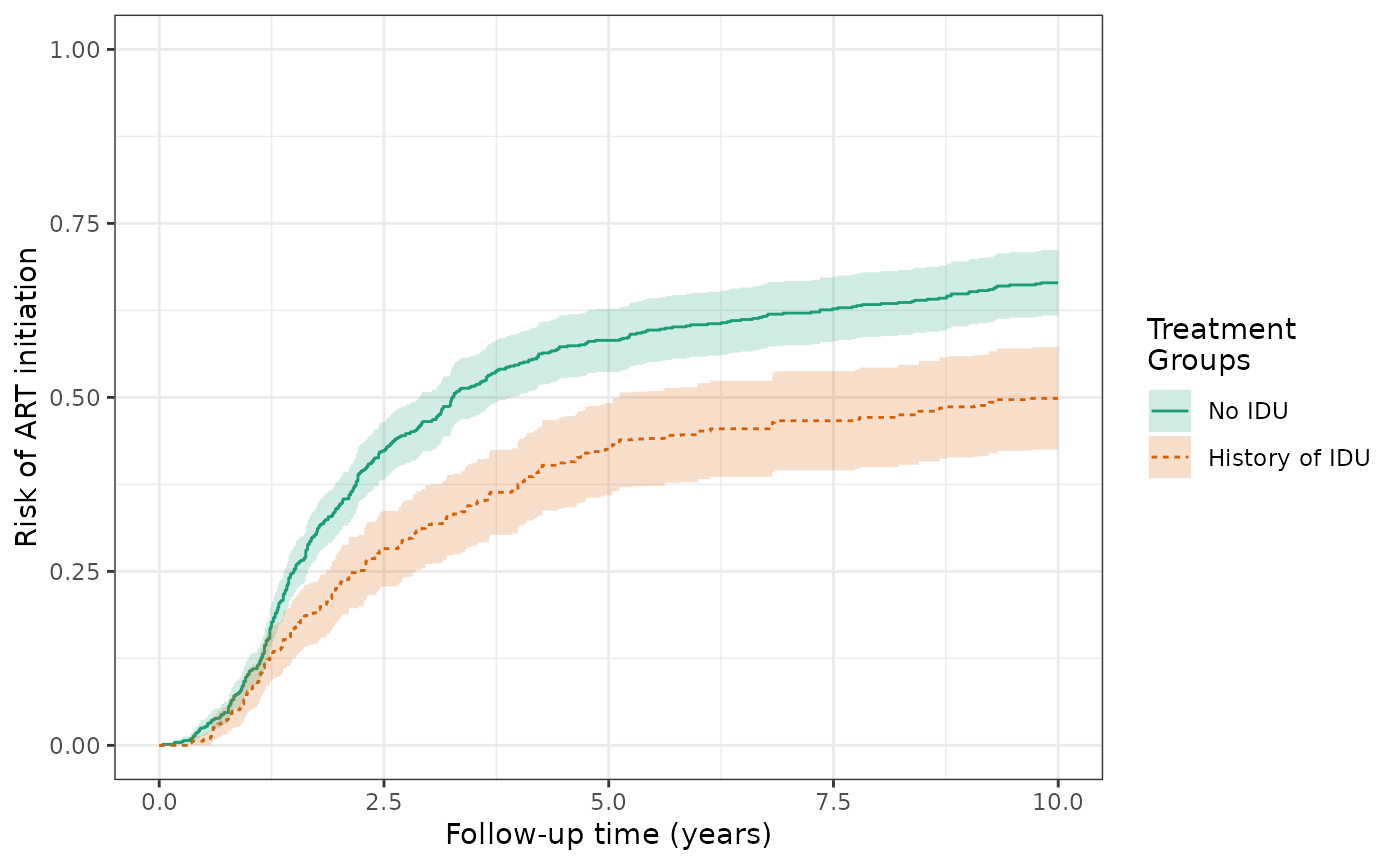
make_table2(wihs4_art_smr, risk_time = 10)The SMR-weighted risks of the AIDS/death outcome (prior to ART initiation) at 10 years are 43.0% for the exposed and 24.1% for the unexposed, with a cumulative risk difference of 18.9%. This risk difference represents the effect of the exposure among the exposed and is slightly increased in magnitude from the IP weighted RD of 16.5%, which was standardized to the total population (rather than just the exposed).
wihs4_aids_smr = estimate_ipwrisk(wihs, ds4_aids,
                         times = seq(0,10,0.01),
                         wt_type = 1,
                         label = c("wihs4 AIDS SMR model"))
plot(wihs4_aids_smr) +
  xlab("Follow-up time (years)") +
  ylab("Risk of AIDS or death") +
  ylim(0,1)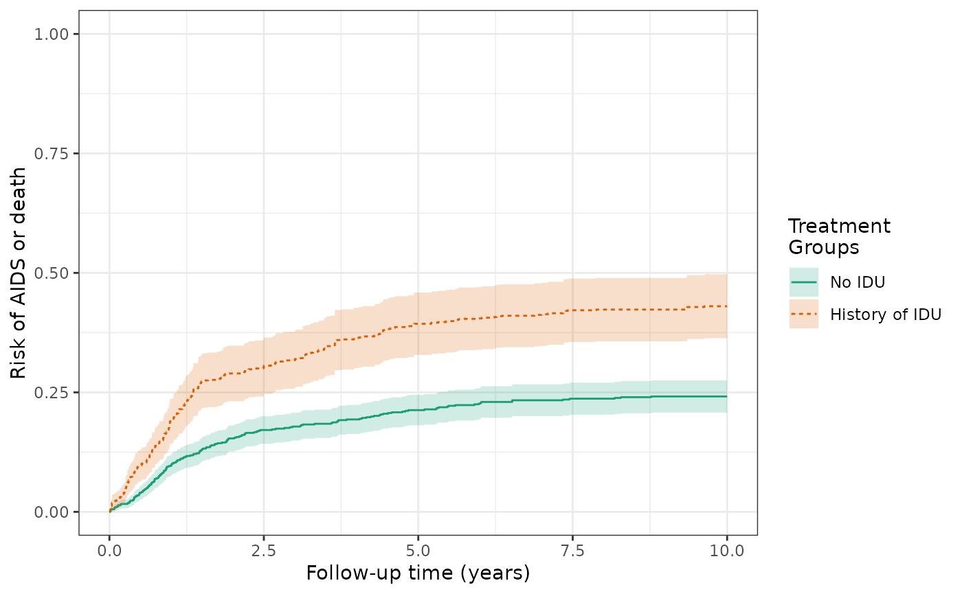
make_table2(wihs4_aids_smr, risk_time = 10)Again, we can compute the weighted means of baseline covariates to understand whether key confounders have been balanced (with unexposed participants now more similar to exposed participants). We can also look at the distribution of weights by exposure group.
make_table1(wihs4_art_smr, white, age, cd4)| Characteristic1 | History of IDU n=1164.00 |
No IDU n=1164.00 |
|---|---|---|
| white | ||
| Non-white Race | 596 51.20 | 641 55.07 |
| White Race | 568 48.80 | 523 44.93 |
| age, Mean (SD) | 36.38 (5.86) | 34.44 (8.46) |
| cd4, Mean (SD) | 379.05 (251.92) | 387.01 (256.32) |
| 1 All values are N (%) unless otherwise specified | ||
make_wt_summary_table(wihs4_art_smr)Model comparison for effect of exposure on the outcome in the total population
This table and plot compares the cumulative risks and RDs from the different models (crude, IPTW, IPTW+IPCW) for the ART initiation outcome.
make_table2(wihs2_art, wihs3_art, wihs4_art, risk_time = 10)
plot(wihs2_art,wihs3_art,wihs4_art, rd=TRUE, overlay=TRUE, legend_title="Models") +
  theme_bw() +
  xlab("Follow-up time (years)") +
ylab("RD for ART initiation by IDU") 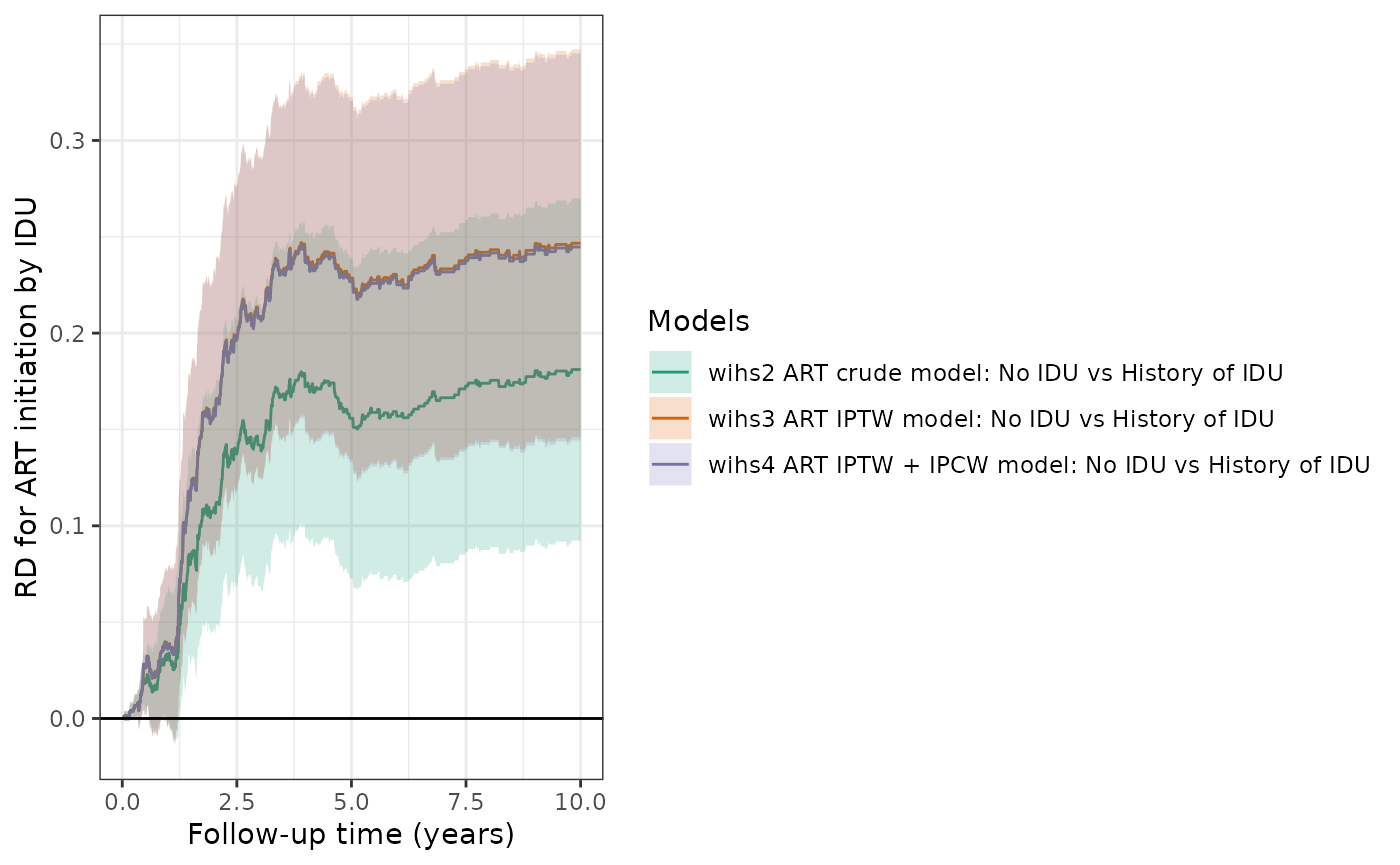
Similarly, this table and plot compare the cumulative risks and RDs from the different models (crude, IPTW, IPTW+IPCW) for the AIDS/death outcome (prior to ART initiation).
make_table2(wihs2_aids, wihs3_aids, wihs4_aids, risk_time = 10)
plot(wihs2_aids, wihs3_aids, wihs4_aids, rd=TRUE, overlay=TRUE, legend_title="Models") +
  theme_bw() +
  xlab("Follow-up time (years)") +
ylab("RD for AIDS/Death by IDU") 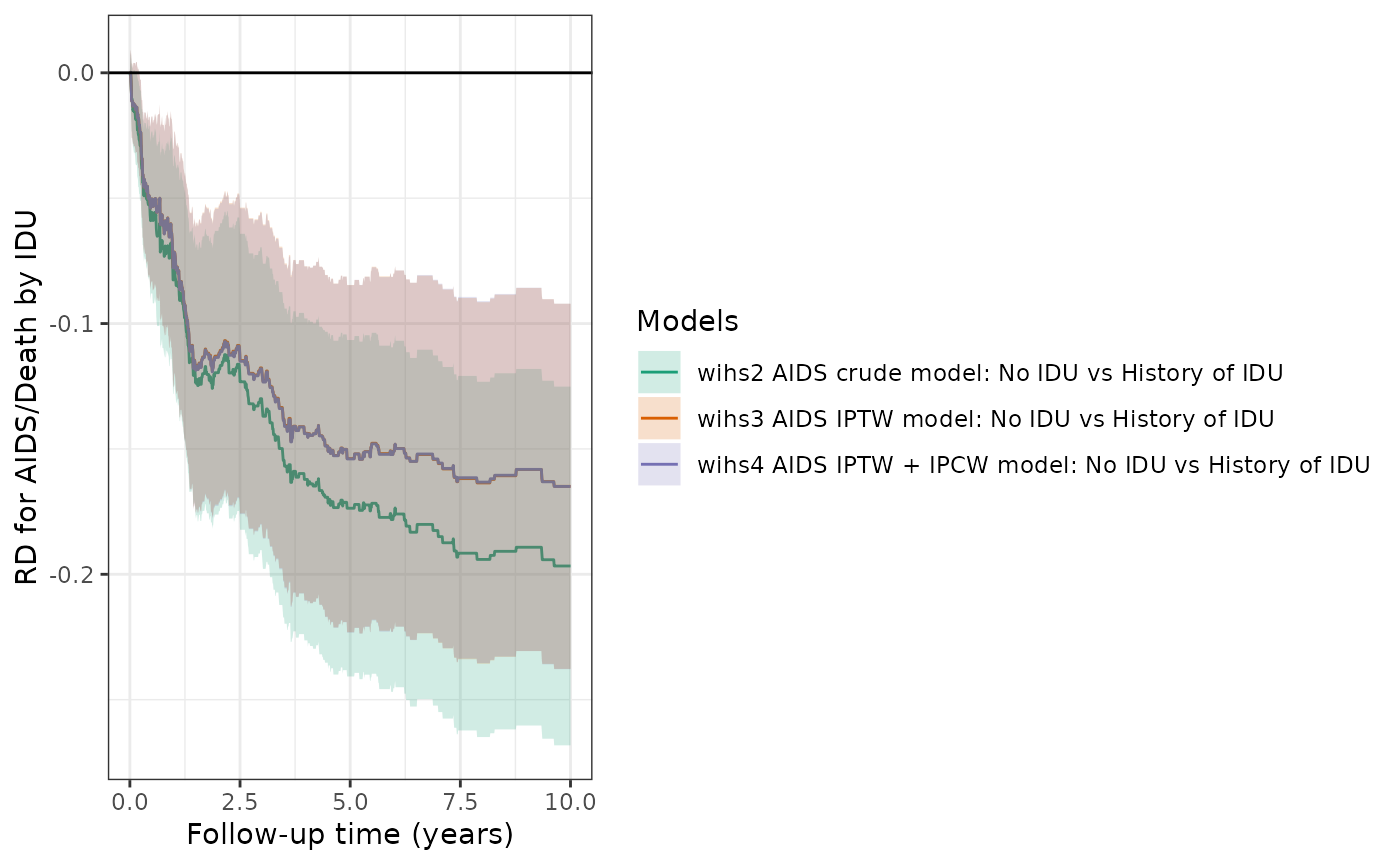
Competing risks
We can estimate the cumulative incidence of ART initiation, factoring in the competing risk of AIDS diagnosis or death. We can respecify the data structure, denoting that the event of interest is ART initiation. The IP-weighted risk of the ART outcome at 10 years are 47.2% for the exposed and 72.7% for the unexposed, and the cumulative risk difference increases in magnitude to -25.5%.
ds5_art = specify_models(
  identify_treatment(idu, formula = ~white+age+cd4),
  identify_censoring(dropout, formula = ~white+age+cd4),
  identify_competing_risk(name = j, event_value = 1),
  identify_outcome(aids_death_art))

wihs5_art = estimate_ipwrisk(wihs, ds5_art,
                        times = seq(0,10,0.01),
                        label = c("wihs risk of ART initiation"))
plot(wihs5_art) +
  theme_bw() +
  xlab("Follow-up time (years)") +
  ylab("Risk of ART initiation") +
  ylim(0,1)
make_table2(wihs5_art, risk_time = 10)For this competing risk analysis, we can plot the cumulative incidence of the composite of both the competing event (AIDS/death prior to ART initiation) and the event of interest (ART initiation), alongside the cumulative incidence of the event of interest and the competing event computed seperately.
ds_composite = specify_models(
  identify_treatment(idu, formula = ~white+age+cd4),
  identify_censoring(dropout, formula = ~white+age+cd4),
  identify_outcome(aids_death_art))

wihs_composite = estimate_ipwrisk(wihs, ds_composite,
                        times = seq(0,10,0.01),
                        label = c("wihs composite outcome"))

ds5_aids = specify_models(
  identify_treatment(idu, formula = ~white+age+cd4),
  identify_censoring(dropout, formula = ~white+age+cd4),
  identify_competing_risk(name = j, event_value = 0),
  identify_outcome(aids_death_art))

wihs5_aids = estimate_ipwrisk(wihs, ds5_aids,
                        times = seq(0,10,0.01),
                        label = c("wihs competing risk"))

plot(wihs_composite, wihs5_art, wihs5_aids, ncol=3, scales="fixed")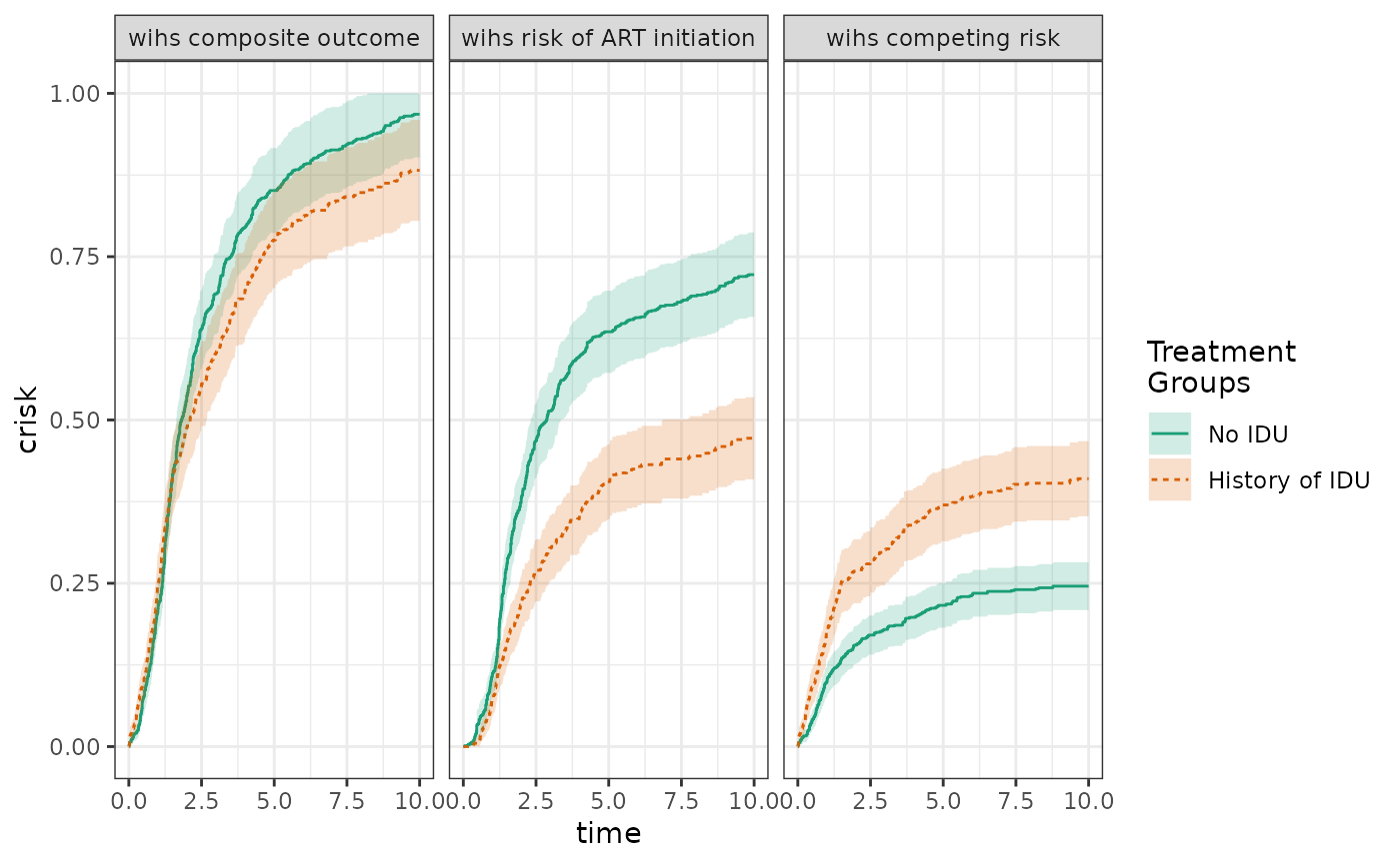
Bootstrap estimation example
Bootstrapping should yield a similar or somewhat narrower confidence band.
wihs5.boot = estimate_ipwrisk(wihs, ds5_art,
                              times=seq(0,10,0.01),
                              label = c("wihs5 bootstrap"), nboot=200)

plot(wihs5_art, wihs5.boot, rd = TRUE, overlay = TRUE, legend_title=" ") +
  theme_bw() +
  ylab("Cumulative Risk Difference") +
xlab("Follow-up time (years)") 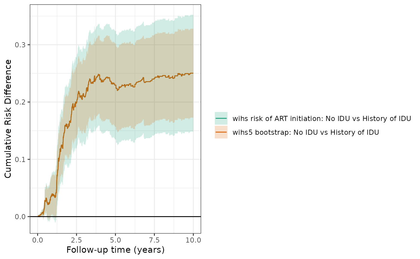
make_table2(wihs5_art, wihs5.boot, risk_time = 10) Sensitivity analysis
We explored the effect of removing race and CD4 count from the propensity score model. We observed little change in the effect estimates when these variables were removed.
wihs5_art %>%
  update_treatment(new_formula = ~.-cd4) %>%
  update_label("Drop CD4 from PS") %>%
  re_estimate ->
  sens1

wihs5_art %>%
  update_treatment(new_formula = ~.-white) %>%
  update_label("Drop white from PS") %>%
  re_estimate ->
  sens2

plot(wihs5_art, sens1, sens2, ncol=3, scales="fixed") + theme_bw() +
  xlab("Follow-up time (years)") +
  ylab("Risk of ART initiation") +
  ylim(0,1)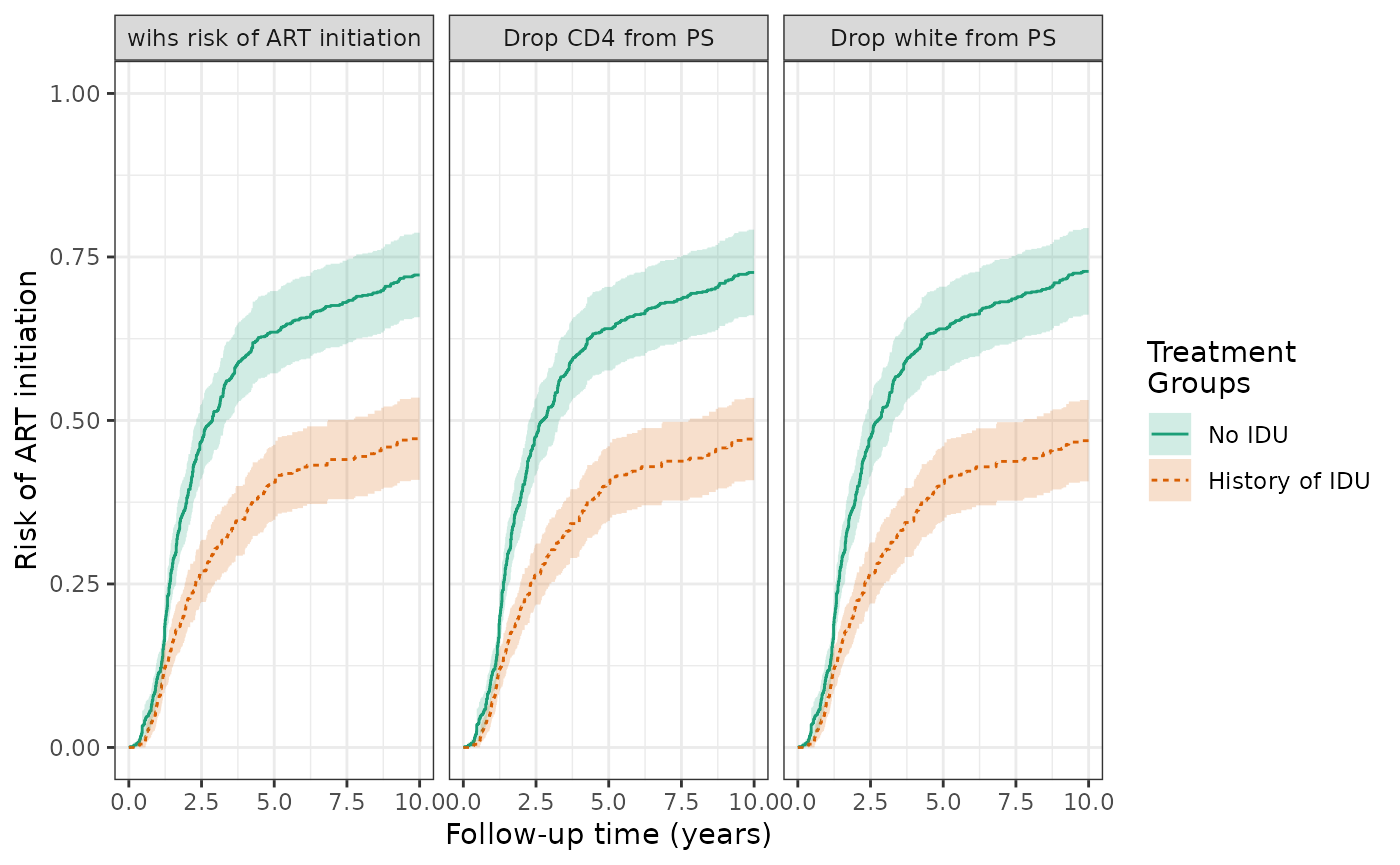
make_table2(wihs5_art, sens1, sens2, risk_time = 10)