Introduction
As described in the “Data Overview” vignette (which should be
reviewed first for required inputs to the nsSank package),
the package supports two workflows for creating Sankey diagrams:
Original Workflow:
With acceptable
eventandcohortdata, the user passes those to thesankey_id_eventsfunction to create anid_dataoutput.-
id_dataandcohortare then passed to either:sankey_list_maker: Converts data into the required JSON format needed to make Sankeys on the Target RWE platformsankey_table_maker: Returns a table with all combinations of states present in the data with corresponding counts and formatted percentages.
Modified Workflow (Recommended):
-
With acceptable
eventandcohortdata, the user can directly pass those to any of the following functions:create_time_varying_data: Convertseventandcohortinto a time-varying dataset, where each row represents a time interval per patient and columns indicate which treatments are active during that interval (supports leveled medications)plot_sankey: Generates Sankey diagrams for visualization in RStudiosankey_counts_table: Tabulates the number of patients in each state at each time pointsankey_transition_counts: Produces a table of transitions between states, showing the starting state, ending state, transition period, and number of patients for each transitionformat_sankey_data: Converts data into the required JSON format needed to make Sankeys on the Target RWE platform
Modified Workflow: Main Functions and Intended Use-Cases
In this section we cover the intended usage for each of the aforementioned functions:
create_time_varying_dataplot_sankeysankey_counts_tablesankey_transition_countsformat_sankey_data
For this section, the following events and
cohort datasets will be used:
events## # A tibble: 190 × 5
## patient_id index_date start end state
## <int> <date> <date> <date> <chr>
## 1 1 2010-06-28 2010-05-08 2010-08-06 A
## 2 1 2010-06-28 2010-07-08 2010-10-06 moderate_intensity_statin
## 3 1 2010-06-28 2010-02-26 2010-04-27 moderate_intensity_statin
## 4 1 2010-06-28 2010-03-12 2010-04-11 moderate_intensity_statin
## 5 1 2010-06-28 2010-12-13 2011-02-11 moderate_intensity_statin
## 6 1 2010-06-28 2010-08-07 2010-11-05 A
## 7 1 2010-06-28 2010-08-29 2010-11-27 A
## 8 2 2010-06-07 2010-10-17 2011-01-15 C
## 9 2 2010-06-07 2010-09-20 2010-11-19 C
## 10 2 2010-06-07 2010-09-24 2010-10-24 low_intensity_statin
## # ℹ 180 more rows
cohort## # A tibble: 40 × 9
## patient_id index_date censor_date discontinue_date death_date sex prior_mi
## <int> <date> <date> <date> <date> <fct> <fct>
## 1 1 2010-06-28 2011-07-07 2011-07-15 NA Female Prior MI
## 2 2 2010-06-07 2010-10-12 2010-11-12 NA Male No Prio…
## 3 3 2010-06-16 2011-05-16 NA NA Male No Prio…
## 4 4 2010-06-18 2010-08-13 NA 2010-08-17 Male No Prio…
## 5 5 2010-06-22 2010-10-09 2011-12-07 NA Male No Prio…
## 6 6 2010-06-11 2012-01-14 2010-09-01 NA Female No Prio…
## 7 7 2010-06-30 2010-12-07 NA NA Male No Prio…
## 8 8 2010-06-02 2011-07-24 NA NA Female Prior MI
## 9 9 2010-06-06 2010-07-07 NA 2010-09-24 Female No Prio…
## 10 10 2010-06-30 2012-09-24 NA 2011-04-29 Female No Prio…
## # ℹ 30 more rows
## # ℹ 2 more variables: age <int>, age_cat <fct>Note that the events data has 4 different treatments:
A, B, and C which are non-leveled
(e.g., a patient is either on treatment A or they’re not on
A) and one leveled statin treatment whose
levels are low_intensity_statin,
moderate_intensity_statin, and
high_intensity_statin and which are displayed in the
state column with the other non-leveled treatments.
1. Creating a Time-Varying Treatment Dataset (Recommend Read Here First)
The functions 2 - 5 above accept a rather large number of arguments.
In order to get a handle on these arguments, it is perhaps most
instructive to start with create_time_varying_data whose
arguments are a subset of the arguments used by the others.
Accepted Arguments
-
events- A long format data frame with one row per treatment episode per patient, containing patient id, treatment name, index date, and treatment start/stop date columns. (See “Data Overview” vignette for more specifics on required format). This is the only function out of the 5 above that requires an index date column in theeventsdata. -
index_var- A string specifying the column name ineventsholding patients’ index dates (default:"index_date") -
tx_name- A string specifying the column name ineventsholding treatment names (default:"tx_name") -
tx_start- A string specifying the column name ineventswith treatment start dates (default:"tx_start") -
tx_stop- A string specifying the column name ineventswith treatment stop dates (default:"tx_stop") -
id_var- A string specifying the column name ineventsholding patient IDs (default:"patient_id") -
med_names_list- A character vector specifying which medications from thetx_namecolumn to include in the analysis. Any medication not in this vector will be ignored. -
stages- A numeric vector specifying time points (days from index date) at which to evaluate medication status. IfNULL(default value), time points are automatically determined from treatment start/stop dates in the data. Example:c(0, 45, 90)checks medication status at baseline, day 45, and day 90. -
on_med_tx_end- A logical value indicating whether a patient is considered on treatment on theirtx_stopdate. IfTRUE,tx_stopis the last day ON treatment (inclusive); ifFALSE,tx_stopis the first day OFF treatment (exclusive). Default:FALSE -
med_levels- A named list of character vectors specifying levels for leveled medications or treatments (e.g.,med_levels = list(statin = c("low_intensity_statin", "moderate_intensity_statin", "high_intensity_statin"))). Any medication name listed here (e.g. statin) must be present inmed_names_list. Medications not listed here but present inmed_names_listare treated as binary (on/off).
Example 1a: Time-Varying Dataset - ignoring leveled statin medication
tv_data = nsSank::create_time_varying_data(
  events = events,
  med_names_list = c("A", "B", "C"), ## No statin medication listed.
  ## "A", "B", and "C" are the only medications tracked
  index_var = "index_date",
  tx_name = "state",
  tx_start = "start",
  tx_stop = "end",
  id_var = "patient_id",
  stages = c(0, 45, 90), ## Check medication status on days 0, 45, and 90
  on_med_tx_end = TRUE ## Patients ON treatment on tx_stop date
)

tv_data
## # A tibble: 108 × 6
## patient_id start stop A_indi B_indi C_indi
## <int> <dbl> <dbl> <chr> <chr> <chr>
## 1 1 0 45 A no_B no_C
## 2 1 45 90 A no_B no_C
## 3 1 90 NA A no_B no_C
## 4 2 0 45 no_A no_B no_C
## 5 2 45 90 no_A no_B no_C
## 6 2 90 NA A no_B no_C
## 7 3 0 45 A B no_C
## 8 3 45 90 no_A B no_C
## 9 3 90 NA no_A no_B no_C
## 10 4 0 45 no_A no_B no_C
## # ℹ 98 more rowsExample 1b: Time-Varying Dataset - incorporating leveled statin medication
tv_data = nsSank::create_time_varying_data(
  events = events,
  med_names_list = c("A", "B", "C", "statin"), ## include statin
  ## Function will look for these levels in tx_name:
  med_levels = list(statin = c("low_intensity_statin",
                               "moderate_intensity_statin",
                               "high_intensity_statin")),
  index_var = "index_date",
  tx_name = "state",
  tx_start = "start",
  tx_stop = "end",
  id_var = "patient_id",
  stages = c(0, 45, 90), # Check medication status on days 0, 45, and 90
  on_med_tx_end = TRUE # Patients ON treatment on tx_stop date
)

tv_data
## # A tibble: 108 × 7
## patient_id start stop statin_indi A_indi B_indi C_indi
## <int> <dbl> <dbl> <chr> <chr> <chr> <chr>
## 1 1 0 45 no_statin A no_B no_C
## 2 1 45 90 moderate_intensity_statin A no_B no_C
## 3 1 90 NA moderate_intensity_statin A no_B no_C
## 4 2 0 45 low_intensity_statin no_A no_B no_C
## 5 2 45 90 low_intensity_statin no_A no_B no_C
## 6 2 90 NA no_statin A no_B no_C
## 7 3 0 45 no_statin A B no_C
## 8 3 45 90 no_statin no_A B no_C
## 9 3 90 NA no_statin no_A no_B no_C
## 10 4 0 45 no_statin no_A no_B no_C
## # ℹ 98 more rowsExample 1c: Dataset with Event-Driven Time Points
When stages = NULL, time points are derived from each
patient’s own treatment history rather than fixed days from index.
Specifically, medication status is evaluated at every unique treatment
start date, stop date, and index date present in the data, producing one
row per resulting interval per patient.
tv_data = nsSank::create_time_varying_data(
  events = events,
  med_names_list = c("A", "B", "C", "statin"), ## include statin
  ## Function will look for these levels in tx_name:
  med_levels = list(statin = c("low_intensity_statin",
                               "moderate_intensity_statin",
                               "high_intensity_statin")),
  index_var = "index_date",
  tx_name = "state",
  tx_start = "start",
  tx_stop = "end",
  id_var = "patient_id",
  stages = NULL, ## allow event-driven time-points
  on_med_tx_end = TRUE # Patients ON treatment on tx_stop date
)

tv_data
## # A tibble: 270 × 7
## patient_id start stop statin_indi A_indi B_indi C_indi
## <int> <dbl> <dbl> <chr> <chr> <chr> <chr>
## 1 1 0 10 no_statin A no_B no_C
## 2 1 10 39 moderate_intensity_statin A no_B no_C
## 3 1 39 40 moderate_intensity_statin A no_B no_C
## 4 1 40 62 moderate_intensity_statin A no_B no_C
## 5 1 62 100 moderate_intensity_statin A no_B no_C
## 6 1 100 130 moderate_intensity_statin A no_B no_C
## 7 1 130 152 no_statin A no_B no_C
## 8 1 152 168 no_statin A no_B no_C
## 9 1 168 228 moderate_intensity_statin no_A no_B no_C
## 10 1 228 NA moderate_intensity_statin no_A no_B no_C
## # ℹ 260 more rows2. Plotting and Formatting Sankey Diagrams
Additional Arguments
In addition to the arguments specified above, each of the functions
plot_sankey, sankey_counts_table,
sankey_transition_counts, and
format_sankey_data accept the following additional
arguments:
-
cohort- a wide-format data frame with one-record-per-id that has at minimum 2 columns: a patient id column and a patient index date column. See “Date Overview” vignette for more details on the exact format. -
stage_labels- a character vector with one label per stage. These labels are used to relabel each numeric stage in thestagesargument (e.g.,stage_labels = c("Baseline", "Day 45", "Day 90")) -
weight- logical. WhenTRUE, applies inverse probability of censoring weights (IPCW) to account for patients censored before the final stage. Rather than raw observed counts, all outputs reflect IPCW-adjusted estimates that better represent the full cohort. Requirescensor_varsto be specified. Default isFALSE. See weighting section for more information. -
censor_vars- named character vector. Variable names incohortthat indicate censoring date. Names are used as state labels (e.g.,censor_vars = c("Censored" = "censor_date")). If unnamed, all censoring states are grouped under “Censored”. -
absorbing_vars- named character vector. Variables incohortthat indicate the date of absorbing states. Names are used as state labels (e.g.,absorbing_vars = c("Death" = "death_date")). -
none- A string. Label for the “empty” (no event) state. Default is"None". -
gofl_formula- formula. Stratifies the Sankey by grouping variables usinggofl. Default isNULL(e.g.,gofl_formula = ~ sex * age_cat). See stratification section for more info. -
collapse_states- named list or named vector. Controls how patients who are on multiple treatments simultaneously are represented. As a named list (e.g.,collapse_states = list("Both Treatments" = c("A", "B"))), you explicitly label co-occurring treatment combinations with a custom name. As a named vector (e.g.,c("A" = "a", "B" = "b")), you assign a priority order — patients on multiple treatments are assigned whichever state appears first in the vector. DefaultNULL. -
collapse_levels- named list. Use this when a treatment in your events data appears at multiple intensity levels (e.g., low, moderate, high dose) and you want to treat all levels as a single state. For example,collapse_levels = list(statin = c("low_intensity_statin", "moderate_intensity_statin", "high_intensity_statin"))combines all statin intensities into onestatinstate. DefaultNULL. -
select_event- A string. How overlapping events are selected at each time point."combine"(default) returns all events;"first"takes the earliest;"last"takes the most recent. -
force- logical. Force transition calculations even if they exceed size guidelines. DefaultFALSE. -
from_tv_meds- logical. Indicates whethereventsis already in time-varying format (output ofcreate_time_varying_data). IfFALSE(default), raw events data is expected andmed_names_listmust be provided.
Basic Examples
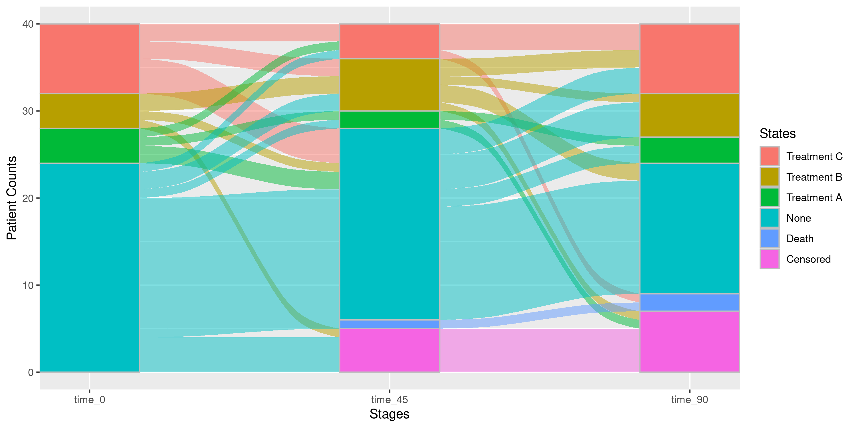
Example 2a: Basic Sankey Diagram with Censoring and Absorbing
nsSank::plot_sankey(
  events = events,
  cohort = cohort,
  med_names_list = c("A", "B", "C"), ## No statin medication listed.
  ## "A", "B", and "C" are the only medications tracked
  index_var = "index_date",
  tx_name = "state",
  tx_start = "start",
  tx_stop = "end",
  id_var = "patient_id",
  stages = c(0, 45, 90), ## Check medication status on days 0, 45, and 90
  on_med_tx_end = TRUE, ## Patients ON treatment on tx_stop date,
  censor_vars = c("Censored" = "censor_date"),
  absorbing_vars = c("Death" = "death_date")
)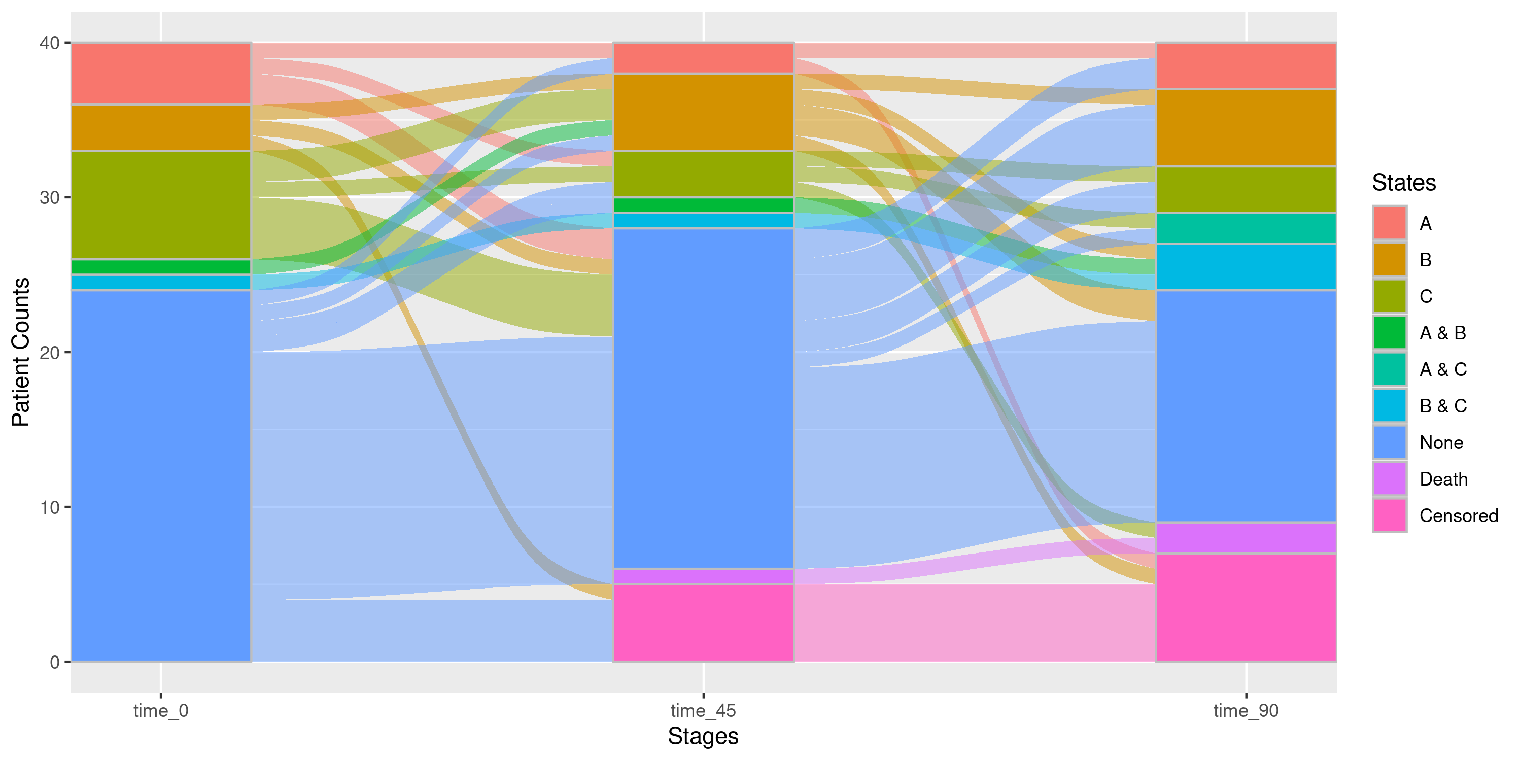
Example 2b: Sankey Diagram with a Leveled Medication
As we noted in example 1a, we did not include statin in
the med_names_list argument, so much like with the
create_time_varying_dataset function, all events where
patients were on any intensity of statin were ignored. If we wish to
incorporate the leveled statin treatment, we must be sure
to include it in med_names_list and specify the levels
using the med_levels argument:
nsSank::plot_sankey(
  events = events,
  cohort = cohort,
  med_names_list = c("A", "B", "C", "statin"), ## Include statin
  med_levels = list(statin = c("low_intensity_statin",
                               "moderate_intensity_statin",
                               "high_intensity_statin")),
  index_var = "index_date",
  tx_name = "state",
  tx_start = "start",
  tx_stop = "end",
  id_var = "patient_id",
  stages = c(0, 45, 90),
  on_med_tx_end = TRUE,
  censor_vars = c("Censored" = "censor_date"),
  absorbing_vars = c("Death" = "death_date")
)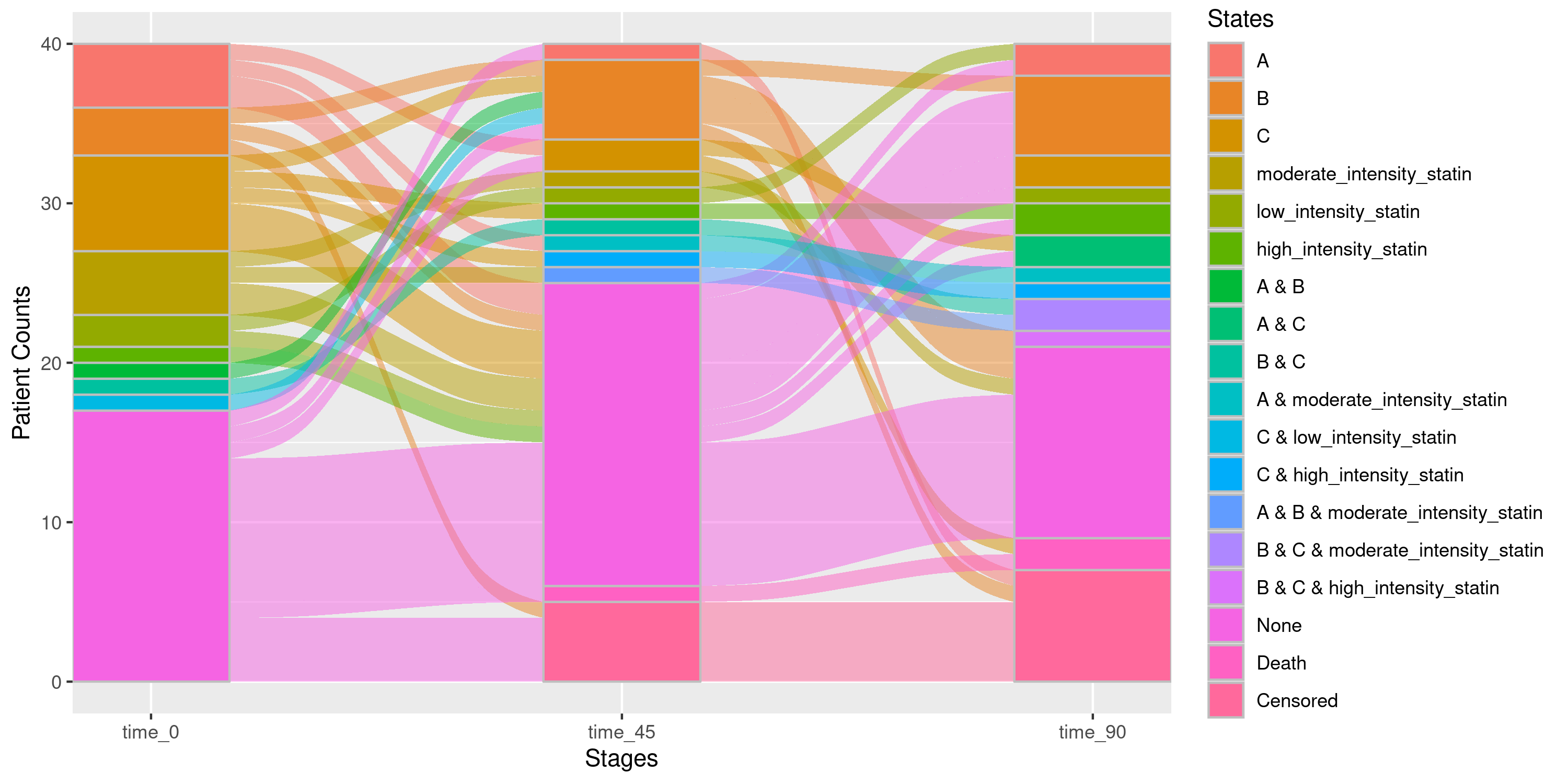
Each level of statin will now be tracked as its own
unique state in the diagram. Of course, this may have the effect of
adding more “clutter” to the diagram, so it may be desirable to simply
collapse these treatment levels and simply have 1 single
statin state to keep track of (i.e. anyone on any intensity
of statin treatment will be considered to be on statin
treatment). We may collapse these medication levels using the
collapse_levels argument:
Example 2c: Sankey Diagram with Collapsed Medication Levels
nsSank::plot_sankey(
  events = events,
  cohort = cohort,
  med_names_list = c("A", "B", "C", "statin"),
  med_levels = list(statin = c("low_intensity_statin",
                               "moderate_intensity_statin",
                               "high_intensity_statin")),
  collapse_levels = list(statin = c("low_intensity_statin",
                                    "moderate_intensity_statin",
                                    "high_intensity_statin")), ## 3 intensities will be collapsed
  index_var = "index_date",
  tx_name = "state",
  tx_start = "start",
  tx_stop = "end",
  id_var = "patient_id",
  stages = c(0, 45, 90),
  on_med_tx_end = TRUE,
  censor_vars = c("Censored" = "censor_date"),
  absorbing_vars = c("Death" = "death_date")
)
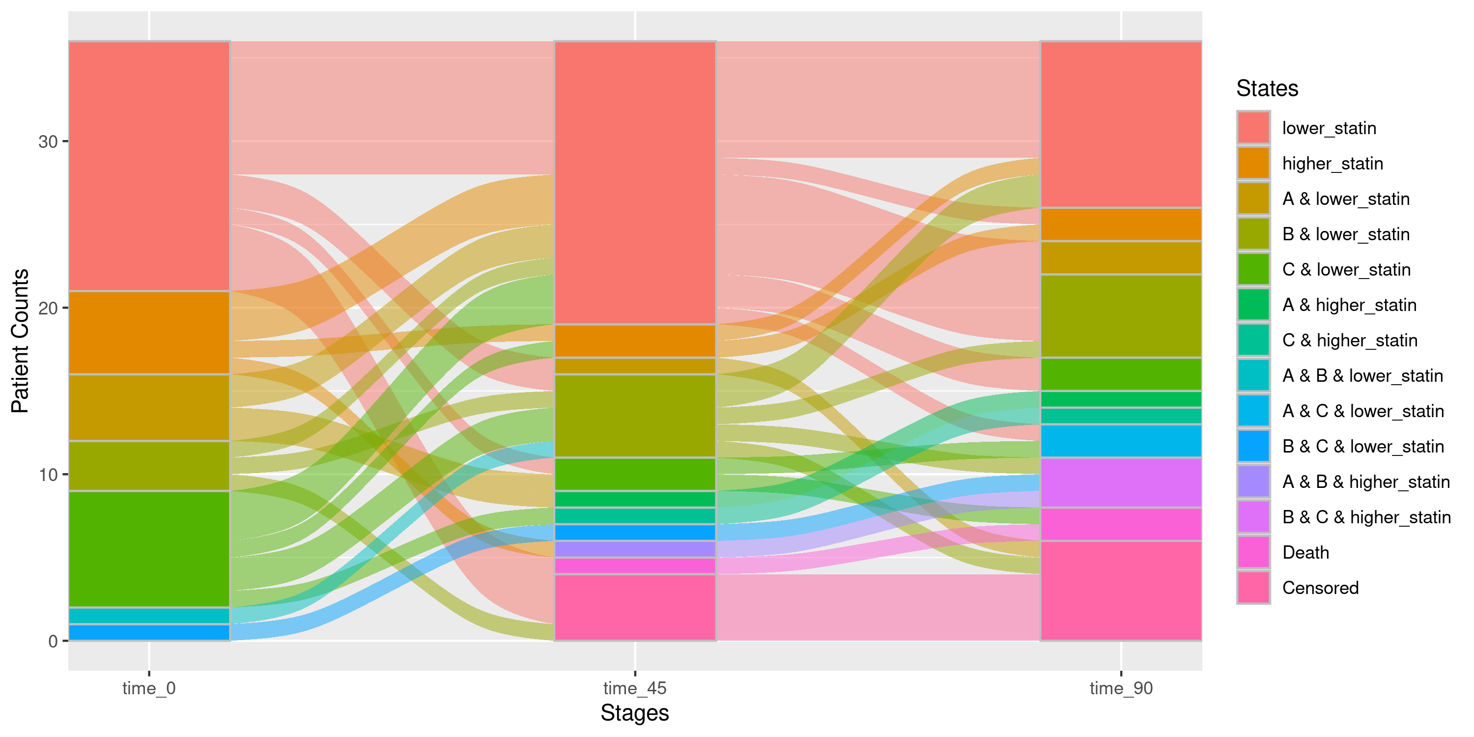
## Let's collapse the statin levels into 2 different states: lower_statin and higher_statin
nsSank::plot_sankey(
  events = events,
  cohort = cohort,
  med_names_list = c("A", "B", "C", "statin"),
  med_levels = list(statin = c("low_intensity_statin",
                               "moderate_intensity_statin",
                               "high_intensity_statin")),
  collapse_levels = list(lower_statin = c("low_intensity_statin",
                                          "no_statin"),
                         higher_statin = c("moderate_intensity_statin",
                                           "high_intensity_statin")),
  index_var = "index_date",
  tx_name = "state",
  tx_start = "start",
  tx_stop = "end",
  id_var = "patient_id",
  stages = c(0, 45, 90),
  on_med_tx_end = TRUE,
  censor_vars = c("Censored" = "censor_date"),
  absorbing_vars = c("Death" = "death_date")
)
Example 2d: Sankey Diagram with Custom Stage Labels
If we want to rename the stage labels, we do so using the
stage_labels argument:
sankey = nsSank::plot_sankey(
  events = events,
  cohort = cohort,
  med_names_list = c("A", "B", "C", "statin"),
  med_levels = list(statin = c("low_intensity_statin",
                               "moderate_intensity_statin",
                               "high_intensity_statin")),
  collapse_levels = list(statin = c("low_intensity_statin",
                                    "moderate_intensity_statin",
                                    "high_intensity_statin")),
  index_var = "index_date",
  tx_name = "state",
  tx_start = "start",
  tx_stop = "end",
  id_var = "patient_id",
  stages = c(0, 45, 90),
  stage_labels = c("Baseline", "Day 45", "Day 90"), ## Renames the stages
  on_med_tx_end = TRUE,
  censor_vars = c("Censored" = "censor_date"),
  absorbing_vars = c("Death" = "death_date")
)

sankey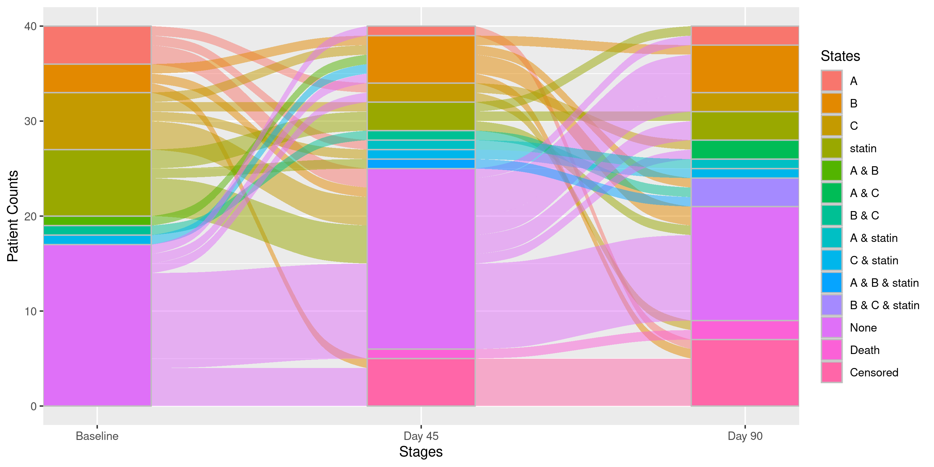
Example 2e: Customizing plot_sankey Output
The output of plot_sankey is a ggplot
object, so standard ggplot2 syntax can be used to adjust
certain elements. However, the degree of customization is limited by how
plot_sankey constructs the plot internally.
Freely customizable via +:
- Plot, Axis and Legend titles - via
labs(x = ..., y = ..., fill = ..., title = ...) - State colors - via
scale_fill_manual()or any otherscale_fill_*function - All theme elements (background, gridlines, font size, legend
position, etc.) - via
theme()
Partially customizable (with caveats):
- Stage axis labels — via
scale_x_discrete(labels = ...), butlimitsmust always be specified and must match the stage column names used internally (i.e., thestage_labelsvalues if set, otherwise"time_0","time_45", etc.). Omittinglimitswill cause axis labels to disappear. - State ordering in the legend and plot - controlled by the factor
level ordering that
plot_sankeysets internally based onstate_map. This cannot be changed after the fact; to reorder states, adjust the order of entries withcollapse_states(see example 4d).
## Same output as example 2d:
sankey = nsSank::plot_sankey(
  events = events,
  cohort = cohort,
  med_names_list = c("A", "B", "C", "statin"),
  med_levels = list(statin = c("low_intensity_statin",
                               "moderate_intensity_statin",
                               "high_intensity_statin")),
  collapse_levels = list(statin = c("low_intensity_statin",
                                    "moderate_intensity_statin",
                                    "high_intensity_statin")),
  index_var = "index_date",
  tx_name = "state",
  tx_start = "start",
  tx_stop = "end",
  id_var = "patient_id",
  stages = c(0, 45, 90),
  stage_labels = c("Baseline", "Day 45", "Day 90"),
  on_med_tx_end = TRUE,
  censor_vars = c("Censored" = "censor_date"),
  absorbing_vars = c("Death" = "death_date")
)

## Let's rename the stages again, rename axes titles, and rename legend title:

sankey +
  labs(x = "Time Points",
       y = "Subject Counts",
       fill = "Treatment Group") +
  scale_x_discrete(limits = c("Baseline", "Day 45", "Day 90"), ## same as user-specified labels
                   labels = c("Baseline" = "Stage 0",
                              "Day 45" = "Stage 1",
                              "Day 90" = "Stage 2"),
                   expand = c(0, 0)) +
  scale_fill_viridis_d() ## Let's go crazy
## Scale for x is already present.
## Adding another scale for x, which will replace the existing scale.
## Scale for fill is already present.
## Adding another scale for fill, which will replace the existing scale.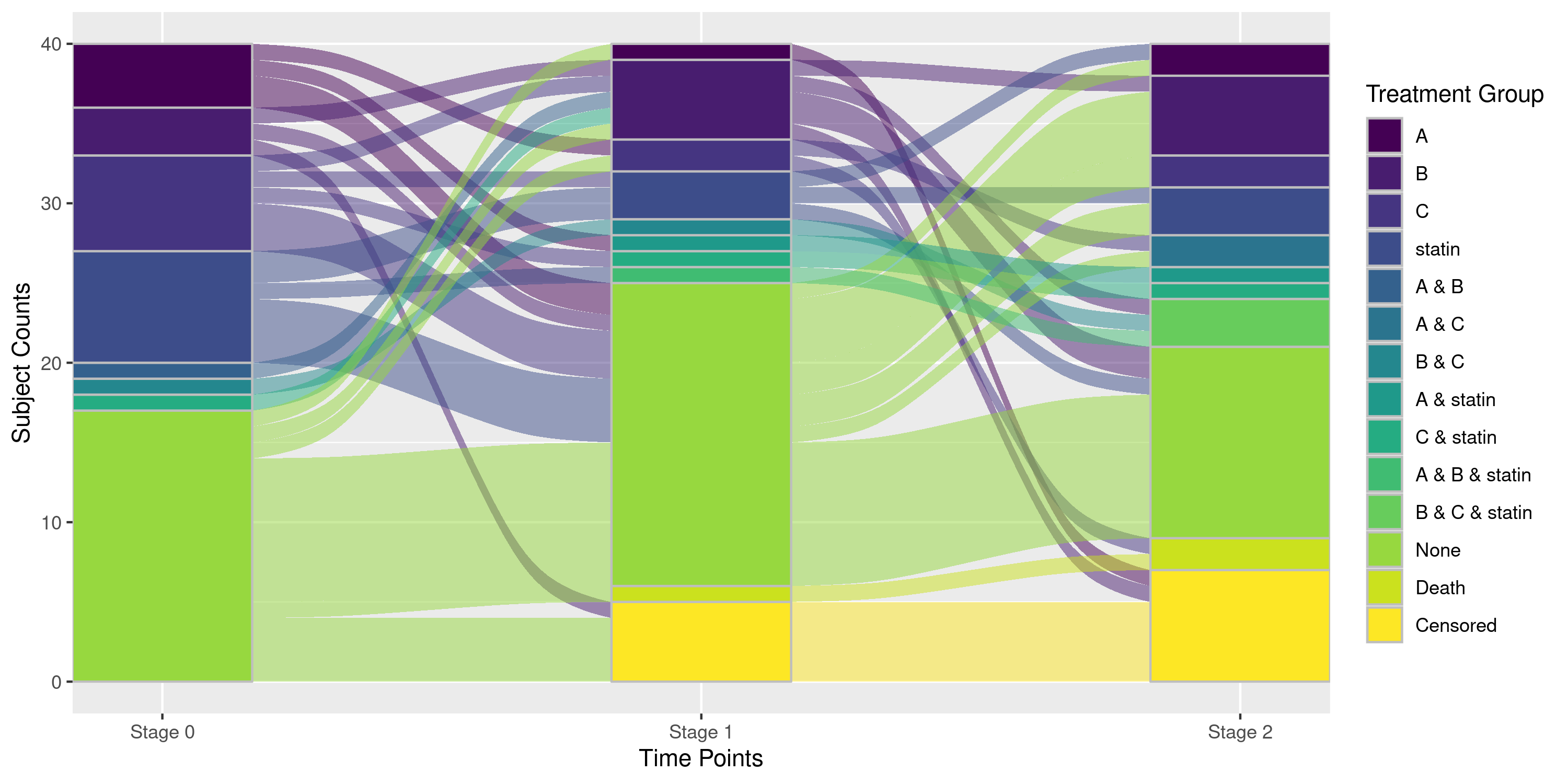
Advanced Features: Weights and Stratification
Creating Weighted Sankey Diagrams
Users have the ability, by setting weight = TRUE, to
create Sankey diagrams that account for patients who are censored before
the final stage. Without weighting, censored patients appear as a
“Censored” state in the diagram, but their counterfactual trajectories
(i.e., what treatment(s) they would have been on had they remained
uncensored) are unaccounted for.
When weight = TRUE, patients who are censored between
stages are up-weighted using inverse probability of censoring weights
(IPCW), so that the remaining observed patients better represent what
the entire cohort would look like had no one been censored. Rather than
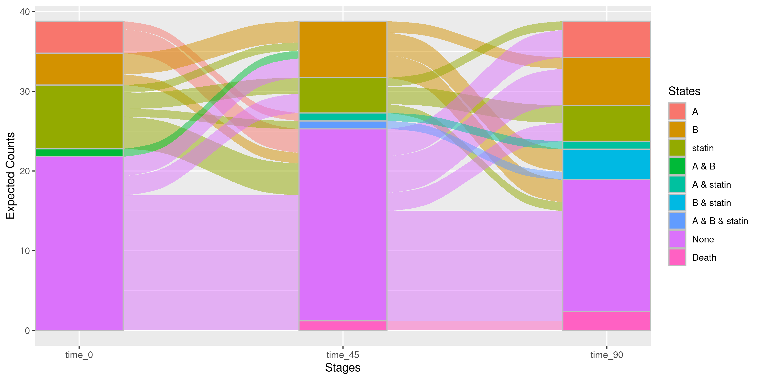
raw patient counts, flow sizes represent IPCW-adjusted expected counts -
estimated as the probability of each treatment pathway multiplied by the
full cohort size. Accordingly, the y-axis label changes from “Patient
Counts” to “Expected Counts”. Note that censor_vars must be
specified for weighting to take effect.
Because the weights are estimated from observed transitions among uncensored patients, pathways that have no observed transitions in the uncensored subset cannot be estimated and are excluded from the diagram. As a result, with small cohorts or high rates of censoring, the expected counts may not sum to the full cohort size.
Note that when weight = TRUE, the function enforces
limits on complexity: no more than 10 states and 8 stages are permitted,
and the total number of possible pathways (states^stages) must not
exceed 1,000,000. These limits exist because computing IPCW-adjusted
transition probabilities scales exponentially with the number of states
and stages. Without weighting, these are warnings rather than errors.
The force = TRUE argument can be used to bypass these
checks, though this is not recommended.
A Weighted Sankey Diagram
nsSank::plot_sankey(
  events = events,
  cohort = cohort,
  med_names_list = c("A", "B", "statin"),
  med_levels = list(statin = c("low_intensity_statin",
                               "moderate_intensity_statin",
                               "high_intensity_statin")),
  collapse_levels = list(statin = c("low_intensity_statin",
                                    "moderate_intensity_statin",
                                    "high_intensity_statin")),
  index_var = "index_date",
  tx_name = "state",
  tx_start = "start",
  tx_stop = "end",
  id_var = "patient_id",
  stages = c(0, 45, 90),
  on_med_tx_end = TRUE,
  censor_vars = c("Censored" = "censor_date"), ## Censoring variables are specified
  absorbing_vars = c("Death" = "death_date"),
  weight = TRUE ## Incorporate weighting
)
Creating Stratified Sankey Diagrams
Should users desire to stratify their Sankey diagrams by certain
categorical variables in their cohort data, they may do so
utilizing the gofl_formula argument. As an example,
consider the following cohort consisting of 2 categorical
variables: sex and age_cat (where patients’
ages have been binned into several categories)
## # A tibble: 40 × 7
##    patient_id index_date censor_date discontinue_date death_date sex    age_cat
##         <int> <date>     <date>      <date>           <date>     <fct>  <fct>
##  1          1 2010-06-28 2011-07-07  2011-07-15       NA         Female (0,40]
##  2          2 2010-06-07 2010-10-12  2010-11-12       NA         Male   (75,90]
##  3          3 2010-06-16 2011-05-16  NA               NA         Male   (75,90]
##  4          4 2010-06-18 2010-08-13  NA               2010-08-17 Male   (0,40]
##  5          5 2010-06-22 2010-10-09  2011-12-07       NA         Male   (0,40]
##  6          6 2010-06-11 2012-01-14  2010-09-01       NA         Female (40,75]
##  7          7 2010-06-30 2010-12-07  NA               NA         Male   (0,40]
##  8          8 2010-06-02 2011-07-24  NA               NA         Female (40,75]
##  9          9 2010-06-06 2010-07-07  NA               2010-09-24 Female (75,90]
## 10         10 2010-06-30 2012-09-24  NA               2011-04-29 Female (40,75]
## # ℹ 30 more rows
Example 3a: Stratifying Sankey Diagrams by each Variable Separately
Specifying gofl_formula = ~ sex + age_cat will produce
marginal groupings: one Sankey per level of sex (filtering
on that level, ignoring age_cat) and one per level of
age_cat (filtering on that level, ignoring
sex), plus an overall, un-stratified Sankey.
By default, if we just set the
gofl_formula = ~ sex + age_cat and call the function, the
output on its own is not immediately useful. When a
gofl_formula is specified by the user, the function returns
a named list with two elements:
-
var_info- a named list mapping each stratification variable to a character vector of its levels -
dt- a list with one element per grouping, where each element is itself a named list containing the stratification variable values for that group along with the Sankey plot (as aggplotobject)
sankey_strat = nsSank::plot_sankey(
  events = events,
  cohort = cohort,
  med_names_list = c("A", "B", "C", "statin"),
  med_levels = list(statin = c("low_intensity_statin",
                               "moderate_intensity_statin",
                               "high_intensity_statin")),
  collapse_levels = list(statin = c("low_intensity_statin",
                                    "moderate_intensity_statin",
                                    "high_intensity_statin")),
  index_var = "index_date",
  tx_name = "state",
  tx_start = "start",
  tx_stop = "end",
  id_var = "patient_id",
  stages = c(0, 45, 90),
  on_med_tx_end = TRUE,
  censor_vars = c("Censored" = "censor_date"),
  absorbing_vars = c("Death" = "death_date"),
  gofl_formula = ~ sex + age_cat
)
Essentially, the output has the following structure:
sankey_strat = list(
  var_info = list(sex = c("Male", "Female"),
                  age_cat = c("(0,40]", "(40,75]","(75,90]")),
  dt = list(
    list(sex = c(NA_character_), age_cat = c(NA_character_), plot = `ggplot`),
    list(sex = c("Male"), age_cat = c(NA_character_), plot = `ggplot`),
    list(sex = c("Female"), age_cat = c(NA_character_), plot = `ggplot`),
    list(sex = c(NA_character_), age_cat = c("(0,40]"), plot = `ggplot`),
    ...
    )
)
To most users, this structure will be unwieldy, so we recommend using
filter_gofl() to extract a specific group from the output
rather than indexing into dt directly. In fact, we can pipe
the output of plot_sankey directly into
filter_gofl to extract our desired strata:
sankey_strat = nsSank::plot_sankey(
  events = events,
  cohort = cohort,
  med_names_list = c("A", "B", "C", "statin"),
  med_levels = list(statin = c("low_intensity_statin",
                               "moderate_intensity_statin",
                               "high_intensity_statin")),
  collapse_levels = list(statin = c("low_intensity_statin",
                                    "moderate_intensity_statin",
                                    "high_intensity_statin")),
  index_var = "index_date",
  tx_name = "state",
  tx_start = "start",
  tx_stop = "end",
  id_var = "patient_id",
  stages = c(0, 45, 90),
  on_med_tx_end = TRUE,
  censor_vars = c("Censored" = "censor_date"),
  absorbing_vars = c("Death" = "death_date"),
  gofl_formula = ~ sex + age_cat
)

## We can just pipe `sankey_strat` into filter_gofl and specify which grouping's Sankey we
## want to view.
## Suppose we wanted to look at the Sankey diagram for everyone that is "Male"
sankey_strat |>
  nsSank::filter_gofl(sex = "Male")
## Let's view the Sankey for everyone that is in the age category (40,75]:
sankey_strat |>
  nsSank::filter_gofl(age_cat = "(40,75]")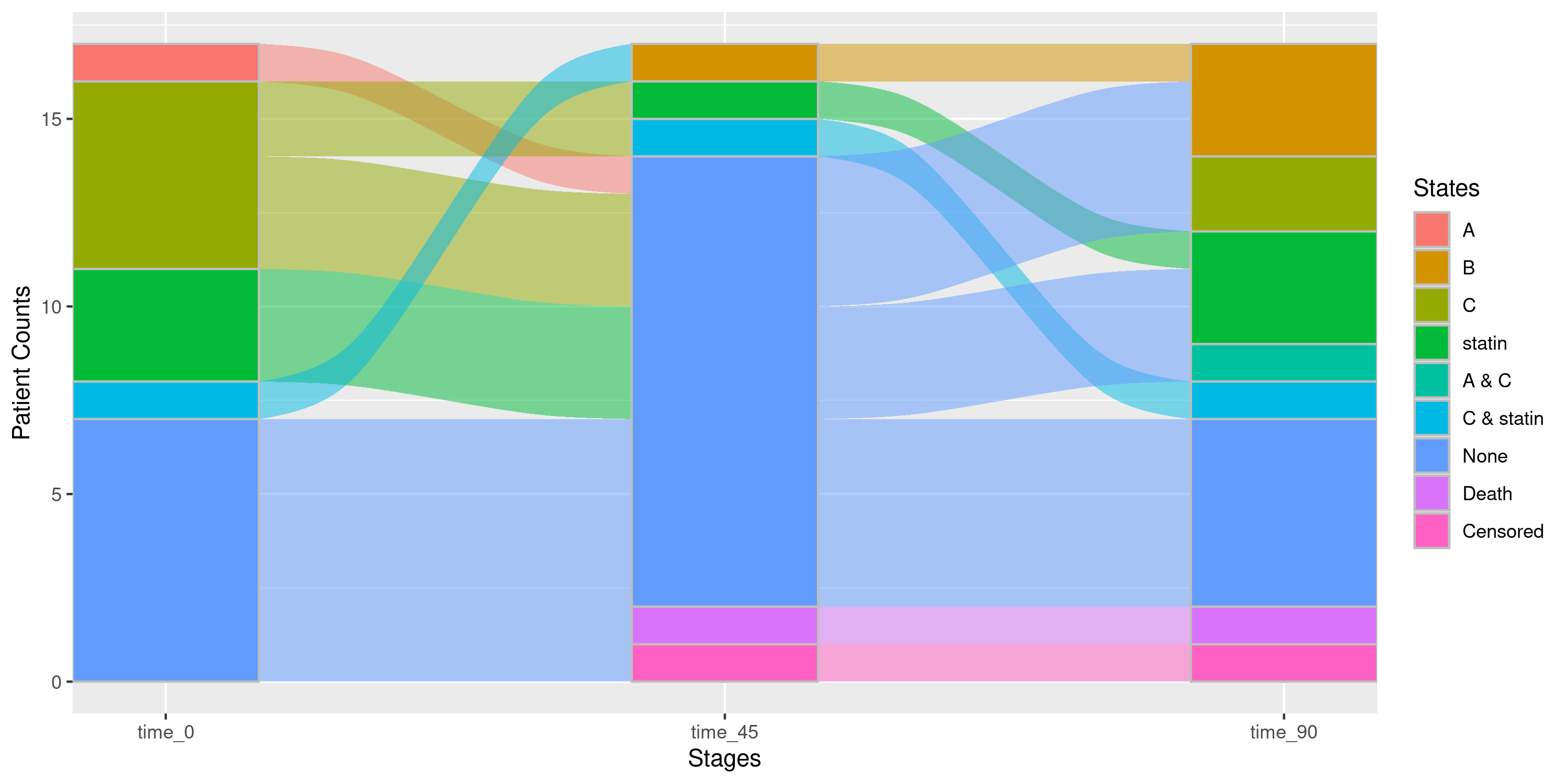
Example 3b: Stratifying Sankey Diagrams by all Combinations
Specifying gofl_formula = ~ sex * age_cat produces all
combinations - every pairing of a sex level with an age category level,
plus the marginals and the overall, un-stratified Sankey.
sankey_strat = nsSank::plot_sankey(
  events = events,
  cohort = cohort,
  med_names_list = c("A", "B", "C", "statin"),
  med_levels = list(statin = c("low_intensity_statin",
                               "moderate_intensity_statin",
                               "high_intensity_statin")),
  collapse_levels = list(statin = c("low_intensity_statin",
                                    "moderate_intensity_statin",
                                    "high_intensity_statin")),
  index_var = "index_date",
  tx_name = "state",
  tx_start = "start",
  tx_stop = "end",
  id_var = "patient_id",
  stages = c(0, 45, 90),
  on_med_tx_end = TRUE,
  censor_vars = c("Censored" = "censor_date"),
  absorbing_vars = c("Death" = "death_date"),
  gofl_formula = ~ sex * age_cat
)

## Let's view the Sankey diagram for all Males in the age category (40,75):
sankey_strat |>
  nsSank::filter_gofl(sex = "Male", age_cat = "(40,75]")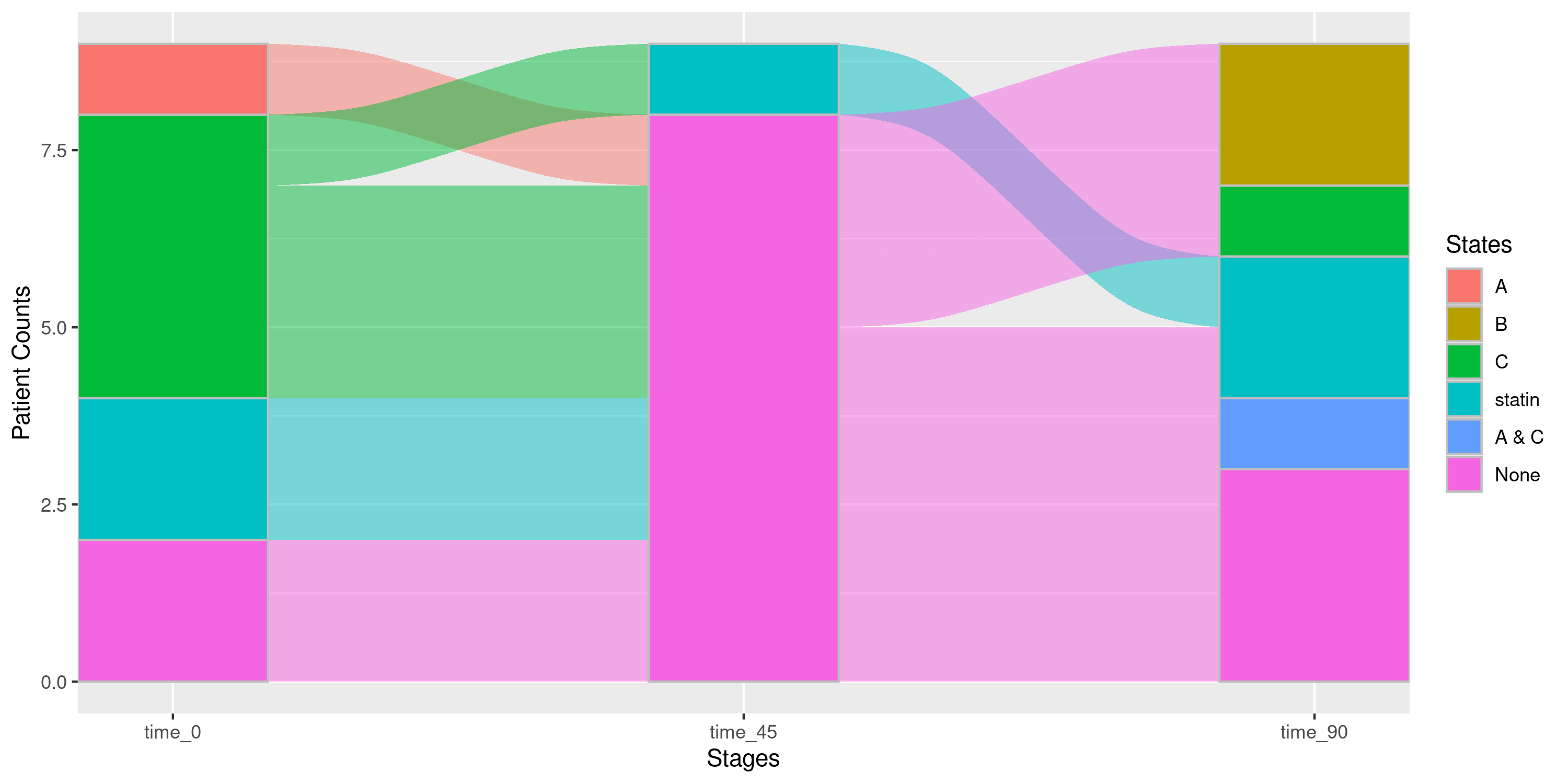
## The Sankey diagram for all males (any age category):
sankey_strat |>
  nsSank::filter_gofl(sex = "Male", age_cat = NA) ## NA is important to specify here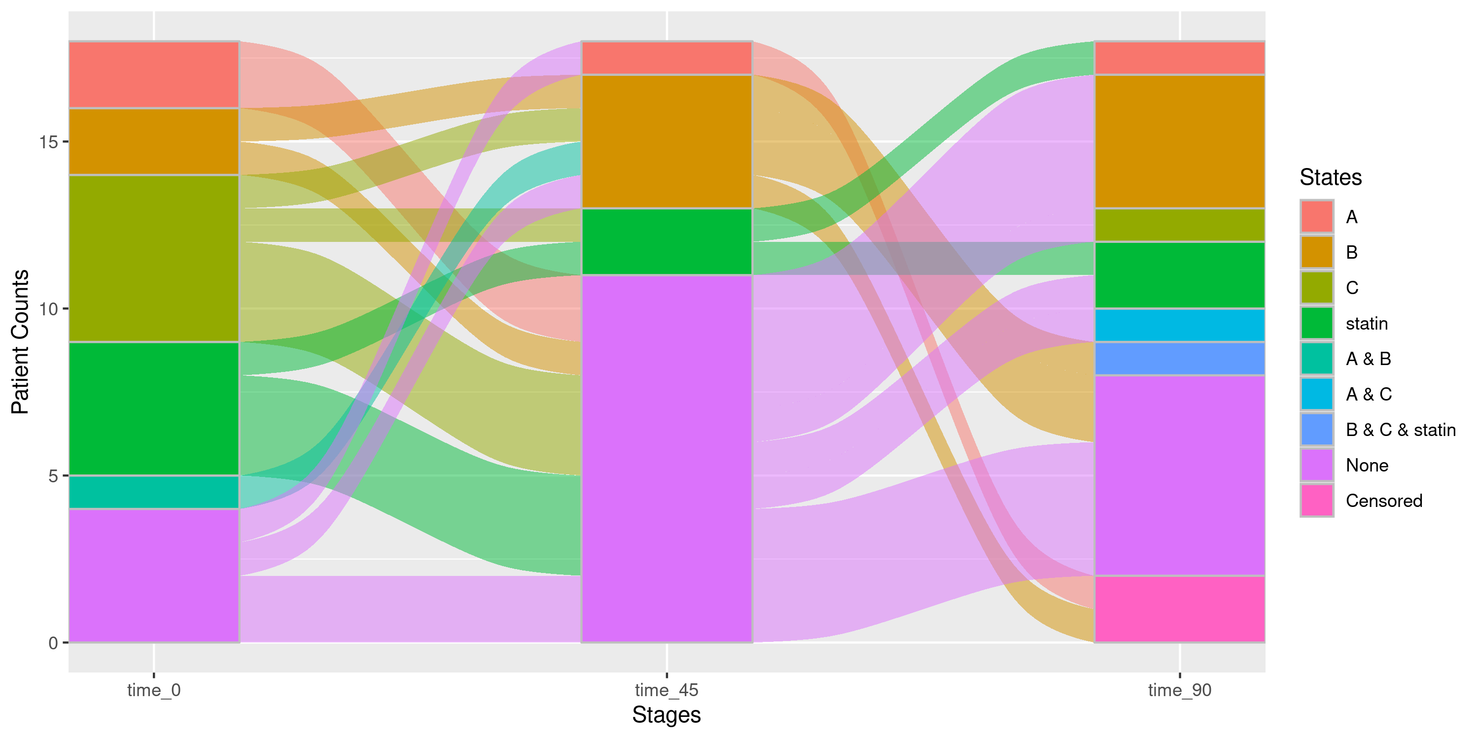
If we only specified sex = "Male" without
age_cat = NA, filter_gofl would return a
partial match - a filtered list containing only the dt
entries where sex = "Male", rather than unwrapping to a
single plot. Our output would look something like this:
sankey_strat |>
  nsSank::filter_gofl(sex = "Male") = list(
    var_info = list(sex = c("Male", "Female"),
                  age_cat = c("(0,40]", "(40,75]","(75,90]")),
    dt = list(
      list(sex = c("Male"), age_cat = c(NA_character_), plot = `ggplot`),
      list(sex = c("Male"), age_cat = c("(0,40]"), plot = `ggplot`),
      list(sex = c("Male"), age_cat = c("(40,75]"), plot = `ggplot`),
      ...
    )
  )
Luckily, if someone has use for this output and then wishes to select a particular age category, they may do so simply by chaining multiple pipe operators:
sankey_strat |>
  nsSank::filter_gofl(sex = "Male") |>
  nsSank::filter_gofl(age_cat = NA)
Arguments: collapse_states
vs. collapse_levels
Both collapse_states and collapse_levels
have the ability to reduce visual clutter in a Sankey Diagram by
flattening 2 or more distinct states into a single state. The question
becomes, what types of states need to be flattened?
We give the following rule of thumb: If one wishes to simply flatten
the intensity levels within medications, it is recommended to
simply use the collapse_levels argument (e.g., see example
2c). However, if one wishes to collapse states across
medications, they must use the collapse_states
argument.
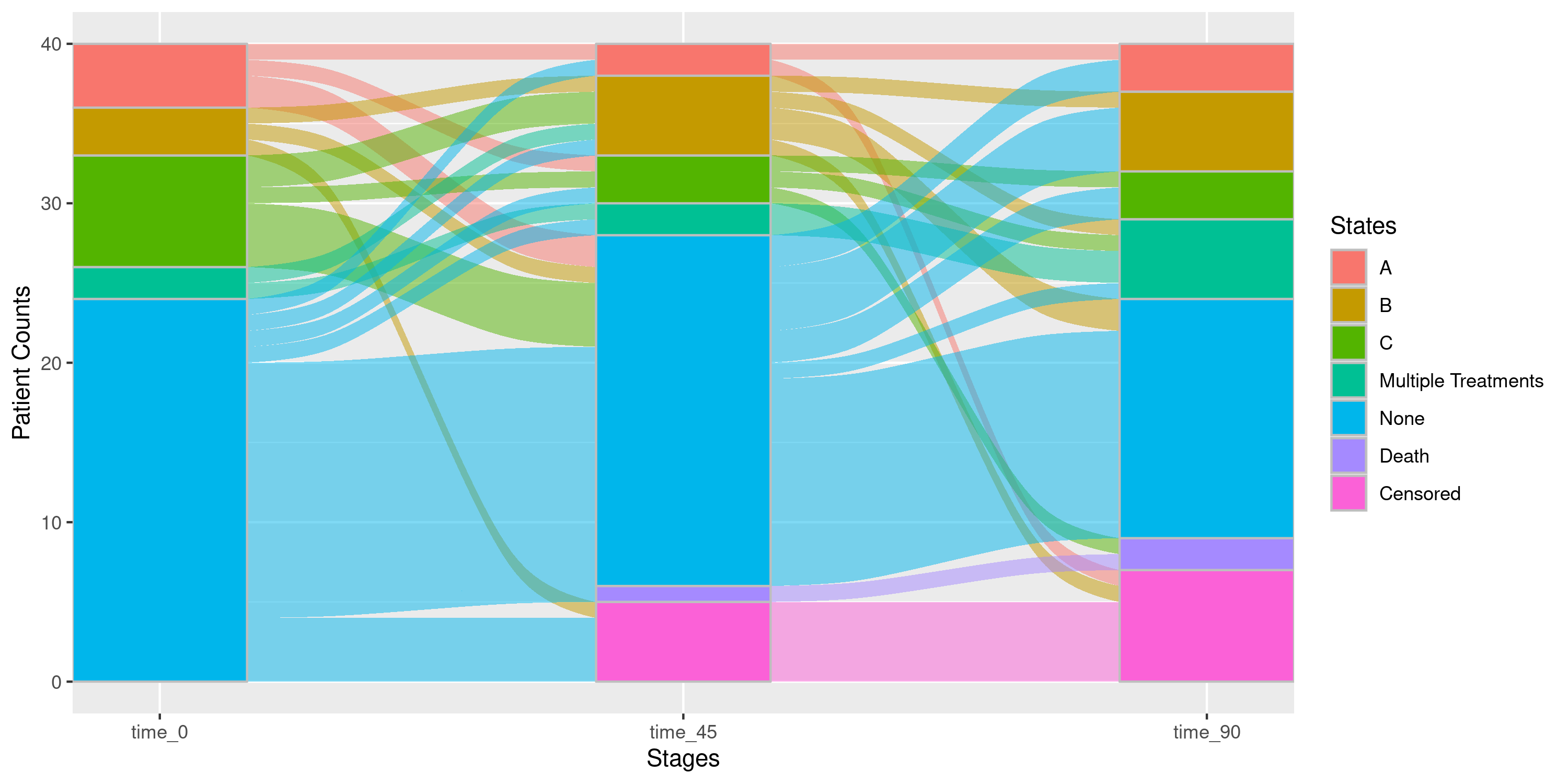
Below, we display patients who are on singular treatments “A”, “B”, or “C”. However, any patient who is on more than 1 of these medications will simply be collapsed into a single “Multiple Treatments” state:
Example 4a: Collapsing Multiple Treatments into a Single State
nsSank::plot_sankey(
  events = events,
  cohort = cohort,
  med_names_list = c("A", "B", "C"),
  collapse_states = list(
    "A" = list("A"),
    "B" = list("B"),
    "C" = list("C"),
    "Multiple Treatments" = list("A & B", "B & C", "A & C", "A & B & C")
  ),
  index_var = "index_date",
  tx_name = "state",
  tx_start = "start",
  tx_stop = "end",
  id_var = "patient_id",
  stages = c(0, 45, 90),
  on_med_tx_end = TRUE,
  censor_vars = c("Censored" = "censor_date"),
  absorbing_vars = c("Death" = "death_date")
)
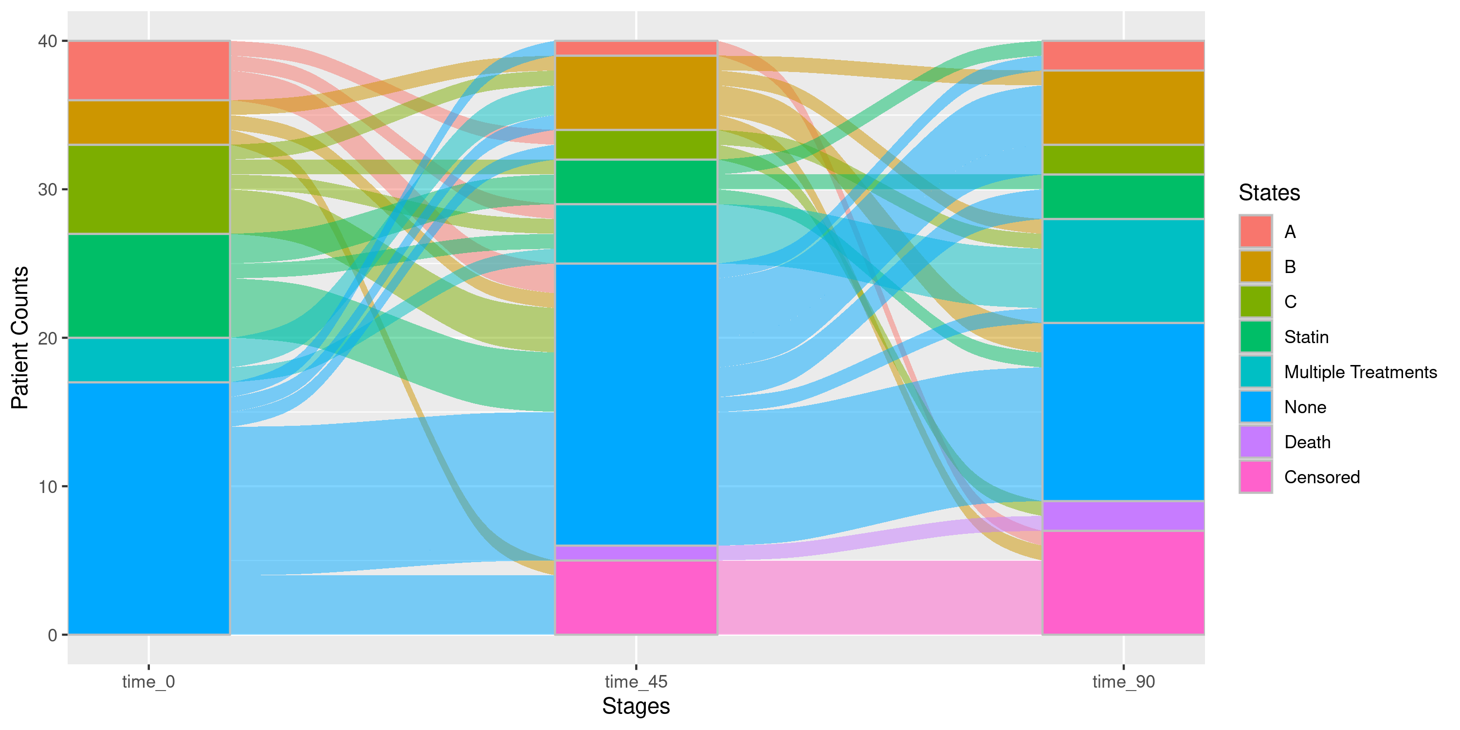
Example 4b: Using both collapse_states and
collapse_levels Simultaneously
As a slightly more complex version of example 4a, suppose we also
want to include a statin medication in our Sankey. In
previous examples, we’ve seen how our events data has 3
statin intensity levels: low_intensity_statin,
moderate_intensity_statin, and
high_intensity_statin. If we want to both collapse these
levels into a single “statin” state while also collapsing states where
patients are on more than 1 treatment simultaneously into a single
“Multiple Treatments” state, we would do so as follows:
- Set the
med_levelsargument which letsnsSankknow what the intensity levels ofstatinare in the first place - Set the
collapse_levelsargument which lets the package know how the user wants to collapse the levels (in our example, any intensity of statin medication will be collapsed to a single “statin” state). - Make sure to specify in
collapse_statesthe basestatinstate and the additional possible combinations of statins may have with the other base treatments “A”, “B”, and “C”. Don’t worry if you miss a combination: the package will return an error informing you which combined states you’ve missed and need to be accounted for.
nsSank::plot_sankey(
  events = events,
  cohort = cohort,
  med_names_list = c("A", "B", "C", "Statin"),
  collapse_states = list(
    "A" = list("A"),
    "B" = list("B"),
    "C" = list("C"),
    "Statin" = list("Statin"),
    "Multiple Treatments" = list("A & B", "B & C", "A & C", "A & B & C",
                                 ## Additional combinations
                                 "A & Statin", "B & Statin", "C & Statin",
                                 "A & B & Statin", "A & C & Statin", "B & C & Statin",
                                 "A & B & C & Statin")
  ),
  med_levels = list(Statin = c("low_intensity_statin",
                               "moderate_intensity_statin",
                               "high_intensity_statin")),
  collapse_levels = list(Statin = c("low_intensity_statin",
                                    "moderate_intensity_statin",
                                    "high_intensity_statin")),
  index_var = "index_date",
  tx_name = "state",
  tx_start = "start",
  tx_stop = "end",
  id_var = "patient_id",
  stages = c(0, 45, 90),
  on_med_tx_end = TRUE,
  censor_vars = c("Censored" = "censor_date"),
  absorbing_vars = c("Death" = "death_date")
)
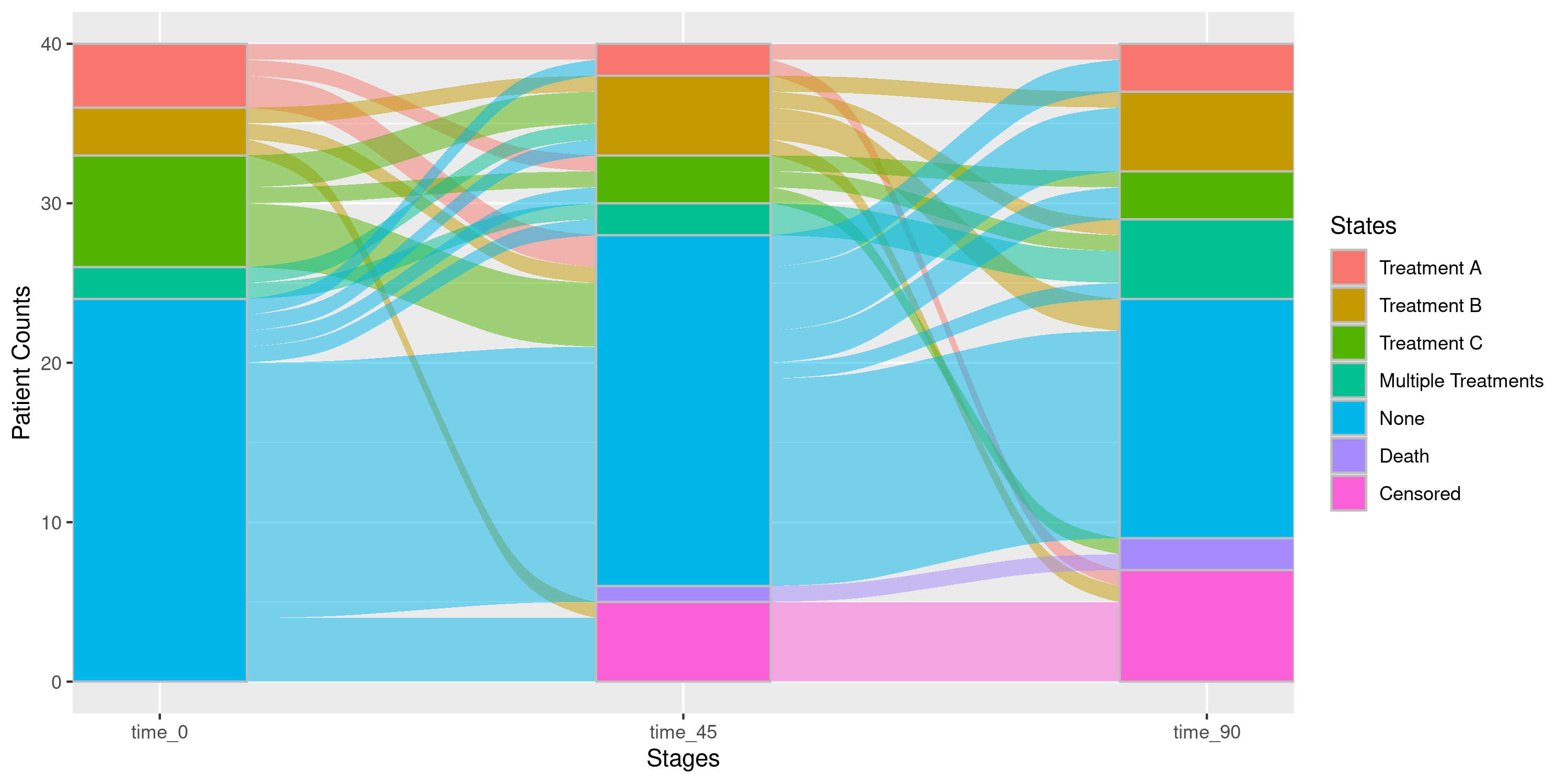
Example 4c: Renaming States Using collapse_states
We can also take this as an opportunity to rename the state labels “A”, “B”, and “C” as “Treatment A”, “Treatment B”, and “Treatment C” if so desired:
nsSank::plot_sankey(
  events = events,
  cohort = cohort,
  med_names_list = c("A", "B", "C"),
  collapse_states = list(
    "Treatment A" = list("A"),
    "Treatment B" = list("B"),
    "Treatment C" = list("C"),
    "Multiple Treatments" = list("A & B", "B & C", "A & C", "A & B & C")
  ),
  index_var = "index_date",
  tx_name = "state",
  tx_start = "start",
  tx_stop = "end",
  id_var = "patient_id",
  stages = c(0, 45, 90),
  on_med_tx_end = TRUE,
  censor_vars = c("Censored" = "censor_date"),
  absorbing_vars = c("Death" = "death_date")
)
Example 4d: Re-ordering States Using
collapse_states
If the user desires to re-order the way states are presented, they
may do so by passing a named character vector to the
collapse_states argument. The order in which the base
states appear in the vector is the order that will be displayed in the
Sankey diagram. For instance, if we want the order to be “Treatment C”
followed by “Treatment B” and then by “Treatment A”, we would specify it
as follows:
nsSank::plot_sankey(
  events = events,
  cohort = cohort,
  med_names_list = c("A", "B", "C"),
  collapse_states = c(
    "Treatment C" = "C",
    "Treatment B" = "B",
    "Treatment A" = "A"
  ),
  index_var = "index_date",
  tx_name = "state",
  tx_start = "start",
  tx_stop = "end",
  id_var = "patient_id",
  stages = c(0, 45, 90),
  on_med_tx_end = TRUE,
  censor_vars = c("Censored" = "censor_date"),
  absorbing_vars = c("Death" = "death_date")
)
Formatting Sankey Diagrams for Target RWE Platform
Once the user is satisfied with the display of their Sankey and
wishes to format it for use on the platform, they simply need to pass in
the same arguments they used for plot_sankey into the
format_sankey_data function. As an example, suppose we were
satisfied with the Sankey diagram in example 4d; we need only copy and
paste the same arguments into the formatting function:
formatted_sankey = nsSank::format_sankey_data(
  events = events,
  cohort = cohort,
  med_names_list = c("A", "B", "C"),
  collapse_states = c(
    "Treatment C" = "C",
    "Treatment B" = "B",
    "Treatment A" = "A"
  ),
  index_var = "index_date",
  tx_name = "state",
  tx_start = "start",
  tx_stop = "end",
  id_var = "patient_id",
  stages = c(0, 45, 90),
  on_med_tx_end = TRUE,
  censor_vars = c("Censored" = "censor_date"),
  absorbing_vars = c("Death" = "death_date")
)
The output is in the same JSON format produced by
sankey_list_maker in the original workflow.
3. Functions for State and Transitions Counts
The two counts functions, sankey_counts_table and
sankey_transition_counts accept the same arguments as
plot_sankey and are used in exactly the same way — the only
difference is what they return. Rather than repeating the argument
descriptions, this section mirrors the examples from Section 2 so users
can directly compare outputs across all three functions for the same
inputs.
Basic Examples (sankey_counts_table)
Example: Basic Counts Table with Censoring and Absorbing
nsSank::sankey_counts_table(
  events = events,
  cohort = cohort,
  med_names_list = c("A", "B", "C"), ## No statin medication listed.
  ## "A", "B", and "C" are the only medications tracked
  index_var = "index_date",
  tx_name = "state",
  tx_start = "start",
  tx_stop = "end",
  id_var = "patient_id",
  stages = c(0, 45, 90), ## Check medication status on days 0, 45, and 90
  on_med_tx_end = TRUE, ## Patients ON treatment on tx_stop date,
  censor_vars = c("Censored" = "censor_date"),
  absorbing_vars = c("Death" = "death_date")
)
## # A tibble: 9 × 4
## state time_0 time_45 time_90
## <chr> <int> <int> <int>
## 1 A 4 2 3
## 2 B 3 5 5
## 3 C 7 3 3
## 4 A & B 1 1 0
## 5 A & C 0 0 2
## 6 B & C 1 1 3
## 7 None 24 22 15
## 8 Death 0 1 2
## 9 Censored 0 5 7Example: State Counts Table with a Leveled Medication
nsSank::sankey_counts_table(
  events = events,
  cohort = cohort,
  med_names_list = c("A", "B", "C", "statin"), ## Include statin
  med_levels = list(statin = c("low_intensity_statin",
                               "moderate_intensity_statin",
                               "high_intensity_statin")),
  index_var = "index_date",
  tx_name = "state",
  tx_start = "start",
  tx_stop = "end",
  id_var = "patient_id",
  stages = c(0, 45, 90),
  on_med_tx_end = TRUE,
  censor_vars = c("Censored" = "censor_date"),
  absorbing_vars = c("Death" = "death_date")
)
## # A tibble: 19 × 4
## state time_0 time_45 time_90
## <chr> <int> <int> <int>
## 1 A 4 1 2
## 2 B 3 5 5
## 3 C 6 2 2
## 4 moderate_intensity_statin 4 1 0
## 5 low_intensity_statin 2 1 1
## 6 high_intensity_statin 1 1 2
## 7 A & B 1 0 0
## 8 A & C 0 0 2
## 9 B & C 1 1 0
## 10 A & moderate_intensity_statin 0 1 1
## 11 B & low_intensity_statin 0 0 0
## 12 C & low_intensity_statin 1 0 0
## 13 C & high_intensity_statin 0 1 1
## 14 A & B & moderate_intensity_statin 0 1 0
## 15 B & C & moderate_intensity_statin 0 0 2
## 16 B & C & high_intensity_statin 0 0 1
## 17 None 17 19 12
## 18 Death 0 1 2
## 19 Censored 0 5 7Example: State Counts Table with Collapsed Medication Levels
nsSank::sankey_counts_table(
  events = events,
  cohort = cohort,
  med_names_list = c("A", "B", "C", "statin"),
  med_levels = list(statin = c("low_intensity_statin",
                               "moderate_intensity_statin",
                               "high_intensity_statin")),
  collapse_levels = list(statin = c("low_intensity_statin",
                                    "moderate_intensity_statin",
                                    "high_intensity_statin")), ## 3 intensities will be collapsed
  index_var = "index_date",
  tx_name = "state",
  tx_start = "start",
  tx_stop = "end",
  id_var = "patient_id",
  stages = c(0, 45, 90),
  on_med_tx_end = TRUE,
  censor_vars = c("Censored" = "censor_date"),
  absorbing_vars = c("Death" = "death_date")
)
## # A tibble: 15 × 4
## state time_0 time_45 time_90
## <chr> <int> <int> <int>
## 1 A 4 1 2
## 2 B 3 5 5
## 3 C 6 2 2
## 4 statin 7 3 3
## 5 A & B 1 0 0
## 6 A & C 0 0 2
## 7 B & C 1 1 0
## 8 A & statin 0 1 1
## 9 B & statin 0 0 0
## 10 C & statin 1 1 1
## 11 A & B & statin 0 1 0
## 12 B & C & statin 0 0 3
## 13 None 17 19 12
## 14 Death 0 1 2
## 15 Censored 0 5 7Example: State Counts Table with Custom Stage Labels
If we want to rename the stage labels, we do so using the
stage_labels argument:
nsSank::sankey_counts_table(
  events = events,
  cohort = cohort,
  med_names_list = c("A", "B", "C", "statin"),
  med_levels = list(statin = c("low_intensity_statin",
                               "moderate_intensity_statin",
                               "high_intensity_statin")),
  collapse_levels = list(statin = c("low_intensity_statin",
                                    "moderate_intensity_statin",
                                    "high_intensity_statin")),
  index_var = "index_date",
  tx_name = "state",
  tx_start = "start",
  tx_stop = "end",
  id_var = "patient_id",
  stages = c(0, 45, 90),
  stage_labels = c("Baseline", "Day 45", "Day 90"), ## Renames the stages
  on_med_tx_end = TRUE,
  censor_vars = c("Censored" = "censor_date"),
  absorbing_vars = c("Death" = "death_date")
)
## # A tibble: 15 × 4
## state Baseline `Day 45` `Day 90`
## <chr> <int> <int> <int>
## 1 A 4 1 2
## 2 B 3 5 5
## 3 C 6 2 2
## 4 statin 7 3 3
## 5 A & B 1 0 0
## 6 A & C 0 0 2
## 7 B & C 1 1 0
## 8 A & statin 0 1 1
## 9 B & statin 0 0 0
## 10 C & statin 1 1 1
## 11 A & B & statin 0 1 0
## 12 B & C & statin 0 0 3
## 13 None 17 19 12
## 14 Death 0 1 2
## 15 Censored 0 5 7Basic Examples (sankey_transition_counts)
Example: Basic Transition Counts with Censoring and Absorbing
nsSank::sankey_transition_counts(
  events = events,
  cohort = cohort,
  med_names_list = c("A", "B", "C"), ## No statin medication listed.
  ## "A", "B", and "C" are the only medications tracked
  index_var = "index_date",
  tx_name = "state",
  tx_start = "start",
  tx_stop = "end",
  id_var = "patient_id",
  stages = c(0, 45, 90), ## Check medication status on days 0, 45, and 90
  on_med_tx_end = TRUE, ## Patients ON treatment on tx_stop date,
  censor_vars = c("Censored" = "censor_date"),
  absorbing_vars = c("Death" = "death_date")
)
## # A tibble: 36 × 4
## from to transition count
## <fct> <fct> <fct> <int>
## 1 A A 0 to 45 1
## 2 A C 0 to 45 1
## 3 A None 0 to 45 2
## 4 B B 0 to 45 1
## 5 B None 0 to 45 1
## 6 B Censored 0 to 45 1
## 7 C B 0 to 45 2
## 8 C C 0 to 45 1
## 9 C None 0 to 45 4
## 10 A & B B 0 to 45 1
## # ℹ 26 more rowsExample: Transition Counts Table with a Leveled Medication
nsSank::sankey_transition_counts(
  events = events,
  cohort = cohort,
  med_names_list = c("A", "B", "C", "statin"), ## Include statin
  med_levels = list(statin = c("low_intensity_statin",
                               "moderate_intensity_statin",
                               "high_intensity_statin")),
  index_var = "index_date",
  tx_name = "state",
  tx_start = "start",
  tx_stop = "end",
  id_var = "patient_id",
  stages = c(0, 45, 90),
  on_med_tx_end = TRUE,
  censor_vars = c("Censored" = "censor_date"),
  absorbing_vars = c("Death" = "death_date")
)
## # A tibble: 48 × 4
## from to transition count
## <fct> <fct> <fct> <int>
## 1 A C 0 to 45 1
## 2 A A & moderate_intensity_statin 0 to 45 1
## 3 A None 0 to 45 2
## 4 B B 0 to 45 1
## 5 B None 0 to 45 1
## 6 B Censored 0 to 45 1
## 7 C B 0 to 45 1
## 8 C high_intensity_statin 0 to 45 1
## 9 C C & high_intensity_statin 0 to 45 1
## 10 C None 0 to 45 3
## # ℹ 38 more rowsExample: Transition Counts with Collapsed Medication Levels
nsSank::sankey_transition_counts(
  events = events,
  cohort = cohort,
  med_names_list = c("A", "B", "C", "statin"),
  med_levels = list(statin = c("low_intensity_statin",
                               "moderate_intensity_statin",
                               "high_intensity_statin")),
  collapse_levels = list(statin = c("low_intensity_statin",
                                    "moderate_intensity_statin",
                                    "high_intensity_statin")), ## 3 intensities will be collapsed
  index_var = "index_date",
  tx_name = "state",
  tx_start = "start",
  tx_stop = "end",
  id_var = "patient_id",
  stages = c(0, 45, 90),
  on_med_tx_end = TRUE,
  censor_vars = c("Censored" = "censor_date"),
  absorbing_vars = c("Death" = "death_date")
)
## # A tibble: 44 × 4
## from to transition count
## <fct> <fct> <fct> <int>
## 1 A C 0 to 45 1
## 2 A A & statin 0 to 45 1
## 3 A None 0 to 45 2
## 4 B B 0 to 45 1
## 5 B None 0 to 45 1
## 6 B Censored 0 to 45 1
## 7 C B 0 to 45 1
## 8 C statin 0 to 45 1
## 9 C C & statin 0 to 45 1
## 10 C None 0 to 45 3
## # ℹ 34 more rowsExample: Transition Counts with Custom Stage Labels
If we want to rename the stage labels, we do so using the
stage_labels argument:
nsSank::sankey_transition_counts(
  events = events,
  cohort = cohort,
  med_names_list = c("A", "B", "C", "statin"),
  med_levels = list(statin = c("low_intensity_statin",
                               "moderate_intensity_statin",
                               "high_intensity_statin")),
  collapse_levels = list(statin = c("low_intensity_statin",
                                    "moderate_intensity_statin",
                                    "high_intensity_statin")),
  index_var = "index_date",
  tx_name = "state",
  tx_start = "start",
  tx_stop = "end",
  id_var = "patient_id",
  stages = c(0, 45, 90),
  stage_labels = c("Baseline", "Day 45", "Day 90"), ## Renames the stages
  on_med_tx_end = TRUE,
  censor_vars = c("Censored" = "censor_date"),
  absorbing_vars = c("Death" = "death_date")
)
## # A tibble: 44 × 4
## from to transition count
## <fct> <fct> <fct> <int>
## 1 A C Baseline to Day 45 1
## 2 A A & statin Baseline to Day 45 1
## 3 A None Baseline to Day 45 2
## 4 B B Baseline to Day 45 1
## 5 B None Baseline to Day 45 1
## 6 B Censored Baseline to Day 45 1
## 7 C B Baseline to Day 45 1
## 8 C statin Baseline to Day 45 1
## 9 C C & statin Baseline to Day 45 1
## 10 C None Baseline to Day 45 3
## # ℹ 34 more rowsAdvanced Features: Weights and Stratification
(sankey_counts_table)
A Weighted State Counts Table
nsSank::sankey_counts_table(
  events = events,
  cohort = cohort,
  med_names_list = c("A", "B", "statin"),
  med_levels = list(statin = c("low_intensity_statin",
                               "moderate_intensity_statin",
                               "high_intensity_statin")),
  collapse_levels = list(statin = c("low_intensity_statin",
                                    "moderate_intensity_statin",
                                    "high_intensity_statin")),
  index_var = "index_date",
  tx_name = "state",
  tx_start = "start",
  tx_stop = "end",
  id_var = "patient_id",
  stages = c(0, 45, 90),
  on_med_tx_end = TRUE,
  censor_vars = c("Censored" = "censor_date"), ## Censoring variables are specified
  absorbing_vars = c("Death" = "death_date"),
  weight = TRUE ## Incorporate weighting
)
## # A tibble: 9 × 4
## state time_0 time_45 time_90
## <chr> <dbl> <dbl> <dbl>
## 1 A 4 0 4.54
## 2 B 4 7.09 6.00
## 3 statin 8 4.42 4.50
## 4 A & B 1 0 0
## 5 A & statin 0 1 1
## 6 B & statin 0 0 3.84
## 7 A & B & statin 0 1 0
## 8 None 21.8 24.1 16.5
## 9 Death 0 1.21 2.36Example 3a: Stratifying State Counts Tables by each Variable Separately
sankey_strat = nsSank::sankey_counts_table(
  events = events,
  cohort = cohort,
  med_names_list = c("A", "B", "C", "statin"),
  med_levels = list(statin = c("low_intensity_statin",
                               "moderate_intensity_statin",
                               "high_intensity_statin")),
  collapse_levels = list(statin = c("low_intensity_statin",
                                    "moderate_intensity_statin",
                                    "high_intensity_statin")),
  index_var = "index_date",
  tx_name = "state",
  tx_start = "start",
  tx_stop = "end",
  id_var = "patient_id",
  stages = c(0, 45, 90),
  on_med_tx_end = TRUE,
  censor_vars = c("Censored" = "censor_date"),
  absorbing_vars = c("Death" = "death_date"),
  gofl_formula = ~ sex + age_cat
)

## We can just pipe `sankey_strat` into filter_gofl and specify which grouping's state counts we
## want to view.
## Suppose we wanted to look at the state counts for everyone that is "Male"
sankey_strat |>
  nsSank::filter_gofl(sex = "Male")
## # A tibble: 15 × 4
## state time_0 time_45 time_90
## <chr> <int> <int> <int>
## 1 A 2 1 1
## 2 B 2 4 4
## 3 C 5 0 1
## 4 statin 4 2 2
## 5 A & B 1 0 0
## 6 A & C 0 0 1
## 7 B & C 0 0 0
## 8 A & statin 0 0 0
## 9 B & statin 0 0 0
## 10 C & statin 0 0 0
## 11 A & B & statin 0 0 0
## 12 B & C & statin 0 0 1
## 13 None 4 11 6
## 14 Death 0 0 0
## 15 Censored 0 0 2
## Let's view the state counts for everyone that is in the age category (40,75]:
sankey_strat |>
  nsSank::filter_gofl(age_cat = "(40,75]")
## # A tibble: 15 × 4
## state time_0 time_45 time_90
## <chr> <int> <int> <int>
## 1 A 1 0 0
## 2 B 0 1 3
## 3 C 5 0 2
## 4 statin 3 1 3
## 5 A & B 0 0 0
## 6 A & C 0 0 1
## 7 B & C 0 0 0
## 8 A & statin 0 0 0
## 9 B & statin 0 0 0
## 10 C & statin 1 1 1
## 11 A & B & statin 0 0 0
## 12 B & C & statin 0 0 0
## 13 None 7 12 5
## 14 Death 0 1 1
## 15 Censored 0 1 1Example 3b: Stratifying State Counts Tables by all Combinations
sankey_strat = nsSank::sankey_counts_table(
  events = events,
  cohort = cohort,
  med_names_list = c("A", "B", "C", "statin"),
  med_levels = list(statin = c("low_intensity_statin",
                               "moderate_intensity_statin",
                               "high_intensity_statin")),
  collapse_levels = list(statin = c("low_intensity_statin",
                                    "moderate_intensity_statin",
                                    "high_intensity_statin")),
  index_var = "index_date",
  tx_name = "state",
  tx_start = "start",
  tx_stop = "end",
  id_var = "patient_id",
  stages = c(0, 45, 90),
  on_med_tx_end = TRUE,
  censor_vars = c("Censored" = "censor_date"),
  absorbing_vars = c("Death" = "death_date"),
  gofl_formula = ~ sex * age_cat
)

## Let's view the state counts for all males in the age category (40,75):
sankey_strat |>
  nsSank::filter_gofl(sex = "Male", age_cat = "(40,75]")
## # A tibble: 15 × 4
## state time_0 time_45 time_90
## <chr> <int> <int> <int>
## 1 A 1 0 0
## 2 B 0 0 2
## 3 C 4 0 1
## 4 statin 2 1 2
## 5 A & B 0 0 0
## 6 A & C 0 0 1
## 7 B & C 0 0 0
## 8 A & statin 0 0 0
## 9 B & statin 0 0 0
## 10 C & statin 0 0 0
## 11 A & B & statin 0 0 0
## 12 B & C & statin 0 0 0
## 13 None 2 8 3
## 14 Death 0 0 0
## 15 Censored 0 0 0
## The state counts table for all males (any age category):
sankey_strat |>
  nsSank::filter_gofl(sex = "Male", age_cat = NA)
## # A tibble: 15 × 4
## state time_0 time_45 time_90
## <chr> <int> <int> <int>
## 1 A 2 1 1
## 2 B 2 4 4
## 3 C 5 0 1
## 4 statin 4 2 2
## 5 A & B 1 0 0
## 6 A & C 0 0 1
## 7 B & C 0 0 0
## 8 A & statin 0 0 0
## 9 B & statin 0 0 0
## 10 C & statin 0 0 0
## 11 A & B & statin 0 0 0
## 12 B & C & statin 0 0 1
## 13 None 4 11 6
## 14 Death 0 0 0
## 15 Censored 0 0 2Advanced Features: Weights and Stratification
(sankey_transition_counts)
A Weighted Transition Counts Table
nsSank::sankey_transition_counts(
  events = events,
  cohort = cohort,
  med_names_list = c("A", "B", "statin"),
  med_levels = list(statin = c("low_intensity_statin",
                               "moderate_intensity_statin",
                               "high_intensity_statin")),
  collapse_levels = list(statin = c("low_intensity_statin",
                                    "moderate_intensity_statin",
                                    "high_intensity_statin")),
  index_var = "index_date",
  tx_name = "state",
  tx_start = "start",
  tx_stop = "end",
  id_var = "patient_id",
  stages = c(0, 45, 90),
  on_med_tx_end = TRUE,
  censor_vars = c("Censored" = "censor_date"), # Censoring variables are specified
  absorbing_vars = c("Death" = "death_date"),
  weight = TRUE # Incorporate weighting
)
## # A tibble: 27 × 4
## from to transition count
## <fct> <fct> <fct> <dbl>
## 1 A A & statin 0 to 45 1
## 2 A None 0 to 45 3
## 3 B B 0 to 45 2.67
## 4 B None 0 to 45 1.33
## 5 statin B 0 to 45 1
## 6 statin statin 0 to 45 2
## 7 statin A & B & statin 0 to 45 1
## 8 statin None 0 to 45 4
## 9 A & B B 0 to 45 1
## 10 None B 0 to 45 2.42
## # ℹ 17 more rowsExample 3a: Stratifying Transition Counts by each Variable Separately
sankey_strat = nsSank::sankey_transition_counts(
  events = events,
  cohort = cohort,
  med_names_list = c("A", "B", "C", "statin"),
  med_levels = list(statin = c("low_intensity_statin",
                               "moderate_intensity_statin",
                               "high_intensity_statin")),
  collapse_levels = list(statin = c("low_intensity_statin",
                                    "moderate_intensity_statin",
                                    "high_intensity_statin")),
  index_var = "index_date",
  tx_name = "state",
  tx_start = "start",
  tx_stop = "end",
  id_var = "patient_id",
  stages = c(0, 45, 90),
  on_med_tx_end = TRUE,
  censor_vars = c("Censored" = "censor_date"),
  absorbing_vars = c("Death" = "death_date"),
  gofl_formula = ~ sex + age_cat
)

## We can just pipe `sankey_strat` into filter_gofl and specify which grouping's transition counts we
## want to view.
## Suppose we wanted to look at the transition counts for everyone that is "Male"
sankey_strat |>
  nsSank::filter_gofl(sex = "Male")
## # A tibble: 23 × 4
## from to transition count
## <fct> <fct> <fct> <int>
## 1 A None 0 to 45 2
## 2 B B 0 to 45 1
## 3 B None 0 to 45 1
## 4 C B 0 to 45 1
## 5 C statin 0 to 45 1
## 6 C None 0 to 45 3
## 7 statin statin 0 to 45 1
## 8 statin None 0 to 45 3
## 9 A & B B 0 to 45 1
## 10 None A 0 to 45 1
## # ℹ 13 more rows
## Let's view the transition counts for everyone that is in the age category (40,75]:
sankey_strat |>
  nsSank::filter_gofl(age_cat = "(40,75]")
## # A tibble: 19 × 4
## from to transition count
## <fct> <fct> <fct> <int>
## 1 A None 0 to 45 1
## 2 C statin 0 to 45 1
## 3 C C & statin 0 to 45 1
## 4 C None 0 to 45 3
## 5 statin None 0 to 45 3
## 6 C & statin B 0 to 45 1
## 7 None None 0 to 45 5
## 8 None Death 0 to 45 1
## 9 None Censored 0 to 45 1
## 10 B B 45 to 90 1
## 11 statin statin 45 to 90 1
## 12 C & statin C & statin 45 to 90 1
## 13 None B 45 to 90 2
## 14 None C 45 to 90 2
## 15 None statin 45 to 90 2
## 16 None A & C 45 to 90 1
## 17 None None 45 to 90 5
## 18 Death Death 45 to 90 1
## 19 Censored Censored 45 to 90 1Example 3b: Stratifying Transition Counts Tables by all Combinations
sankey_strat = nsSank::sankey_transition_counts(
  events = events,
  cohort = cohort,
  med_names_list = c("A", "B", "C", "statin"),
  med_levels = list(statin = c("low_intensity_statin",
                               "moderate_intensity_statin",
                               "high_intensity_statin")),
  collapse_levels = list(statin = c("low_intensity_statin",
                                    "moderate_intensity_statin",
                                    "high_intensity_statin")),
  index_var = "index_date",
  tx_name = "state",
  tx_start = "start",
  tx_stop = "end",
  id_var = "patient_id",
  stages = c(0, 45, 90),
  on_med_tx_end = TRUE,
  censor_vars = c("Censored" = "censor_date"),
  absorbing_vars = c("Death" = "death_date"),
  gofl_formula = ~ sex * age_cat
)

## Let's view the transition counts for all males in the age category (40,75):
sankey_strat |>
  nsSank::filter_gofl(sex = "Male", age_cat = "(40,75]")
## # A tibble: 11 × 4
## from to transition count
## <fct> <fct> <fct> <int>
## 1 A None 0 to 45 1
## 2 C statin 0 to 45 1
## 3 C None 0 to 45 3
## 4 statin None 0 to 45 2
## 5 None None 0 to 45 2
## 6 statin statin 45 to 90 1
## 7 None B 45 to 90 2
## 8 None C 45 to 90 1
## 9 None statin 45 to 90 1
## 10 None A & C 45 to 90 1
## 11 None None 45 to 90 3
## The transition counts table for all males (any age category):
sankey_strat |>
  nsSank::filter_gofl(sex = "Male", age_cat = NA)
## # A tibble: 23 × 4
## from to transition count
## <fct> <fct> <fct> <int>
## 1 A None 0 to 45 2
## 2 B B 0 to 45 1
## 3 B None 0 to 45 1
## 4 C B 0 to 45 1
## 5 C statin 0 to 45 1
## 6 C None 0 to 45 3
## 7 statin statin 0 to 45 1
## 8 statin None 0 to 45 3
## 9 A & B B 0 to 45 1
## 10 None A 0 to 45 1
## # ℹ 13 more rowsOriginal Workflow
Overview
To facilitate the partition level data processing, the updates to the
sankey workflow allow for the subject-level calculations to be done in a
separate step from the sankey creation. The only difference now between
the old data formats of the cohort and events
file is that no relative time needs to be calculated–as long as dates
are supplied the package can figure it out.
ID Level Data
First, the id level data are created used
sankey_id_events or sankey_id_ansible. The
only difference is the second argument – sankey_id_events
takes in a data.frame in long format with a start date/ end
date associated with each event. sankey_id_ansible requires
that the second argument is a data.frame in ansible format
(the same format required by sunbursts).
If you aren’t making a sunburst, might as well use
sankey_id_events so you don’t have to deal with the
overhead of converting all the data, which can take awhile.
The idea is that when the cohorts are being created, creating the sankey subject level data can be done on smaller chunks of the data before the necessary summary at the end.
sankey_id_events(cohort,
                 evts,
                 stages,
                 id_var = "patient_id",
                 index_var = "index_date",
                 states = NULL,
                 select_event = "combine")

sankey_id_ansible(cohort,
                  data,
                  stages,
                  id_var = "patient_id",
                  index_var = "index_date",
                  states = NULL,
                  select_event = "combine")
This is to help facilitate running on partitions on the id-level
first, before the summarizing step in sankey_list_maker.
sunburst_id_data requires a cohort, an ansible
style data.frame, and which “states” are wanted. It returns a list of
the resulting data.frame and the states, so it can directly be fed into
sunburst_maker.
Below is an example of the format of the event data, with a start/end date with a corresponding state:
events <- nsSank::convert_tagged_cdf(cdf)
events  %>%
  head() %>%
  rmarkdown::paged_table()
Below is an example of the format of cohort data. An id-level
variable, index date variable, censor date variable,
death_date, and any potential stratification variables.
cohort %>%
  head() %>%
  rmarkdown::paged_table()
Both sankey_id_events and sankey_id_ansible
return a list that contains the id-level data, the identified states,
and the identified stages (timepoints). In the id-level data frame,
states and combinations of states are represented as base2 integers.
sankey_id_data <- nsSank::sankey_id_events(cohort, events, states = c("a", "b", "c"), stages = c(0, 90, 180))You can indicate whether you want the function to choose the first state, last state, or combine overlapping events with . The default is to combine. You can see there aren’t any overlapping events, since we are choosing the most recent prior event instead of combining.
choose_last <- nsSank::sankey_id_events(cohort, events, states = c("a", "b", "c"), stages = c(0, 90, 180), select_event = "last")PHR Sankey Data
Once you have the id-level data, you can summarize and create your sankey list for a PHR. This returns a list of length one, with options needed for the sankey.
sankey_list <- nsSank::sankey_list_maker(sankey_id_data, cohort)You can use the collapse_states argument to specify how
you want overlapping states presented (or for reasons such as changing
the order of the states, or the labels.) The none argument
additionally labels the empty state.
collapse_list <- list(
  "Treatment A" = list("a"),
  "Treatment B" = list("b"),
  "Treatment C" = list("c"),
  "Multiple" = list("a & b", "a & c", "b & c", "a & b & c")
)
sankey_list_collapse <- nsSank::sankey_list_maker(sankey_id_data, cohort, collapse_states = collapse_list, none = "No Treatment")

sankey_list_collapse[[1]]$states
## [1] "Treatment A" "Treatment B" "Treatment C" "Multiple" "No Treatment"If using version 0.2.4 or later, you can specify
collapse_states as a named vector–this will assign a
hierarchy to the combined states and order accordingly:
collapse_vec <- c(
  "Treatment B" = "b",
  "Treatment A" = "a",
  "Treatment C" = "c"
)
sankey_list_collapse <- nsSank::sankey_list_maker(sankey_id_data, cohort, collapse_states = collapse_vec, none = "No Treatment")

sankey_list_collapse[[1]]$states
## [1] "Treatment B" "Treatment A" "Treatment C" "No Treatment"You can also use the stage_labels argument to specify
how you want the time points labelled on the sankey.
sankey_list_collapse_stages <- nsSank::sankey_list_maker(sankey_id_data,
                                                  cohort,
                                                  collapse_states = collapse_list,
                                                  stage_labels = c("Index", "90 Days", "180 Days"))

sankey_list_collapse[[1]]$stages
## [1] "0" "90" "180"Filtered Sankeys
If you want to add filtering to the PHR Sankeys, you can use the
golf_formula argument to specify with what variables and
how you want to be able to filter.
For example, in the cohort we have two categorical
variables we can use: prior_mi and
age_cat.
sankey_list_filtered <- nsSank::sankey_list_maker(sankey_id_data,
                                                  cohort,
                                                  collapse_states = collapse_list,
                                                  stage_labels = c("Index", "90 Days", "180 Days"),
                                                  gofl_formula = ~ prior_mi*age_cat)
That results in a list of lists. The first list var_info
contains descriptive information for the levels of the grouping
variables.
The second list dt contains a list of sankey data for
each level.
prior_mi has 2 levels and age_cat has 3
levels, so we should expect 12 different filter combinations.
purrr::map(sankey_list_filtered$dt, ~.x[1:2])## [[1]]
## [[1]]$prior_mi
## [1] NA
##
## [[1]]$age_cat
## [1] NA
##
##
## [[2]]
## [[2]]$prior_mi
## [1] "No Prior MI"
##
## [[2]]$age_cat
## [1] NA
##
##
## [[3]]
## [[3]]$prior_mi
## [1] "Prior MI"
##
## [[3]]$age_cat
## [1] NA
##
##
## [[4]]
## [[4]]$prior_mi
## [1] NA
##
## [[4]]$age_cat
## [1] "(0,40]"
##
##
## [[5]]
## [[5]]$prior_mi
## [1] NA
##
## [[5]]$age_cat
## [1] "(40,75]"
##
##
## [[6]]
## [[6]]$prior_mi
## [1] NA
##
## [[6]]$age_cat
## [1] "(75,90]"
##
##
## [[7]]
## [[7]]$prior_mi
## [1] "No Prior MI"
##
## [[7]]$age_cat
## [1] "(0,40]"
##
##
## [[8]]
## [[8]]$prior_mi
## [1] "No Prior MI"
##
## [[8]]$age_cat
## [1] "(40,75]"
##
##
## [[9]]
## [[9]]$prior_mi
## [1] "No Prior MI"
##
## [[9]]$age_cat
## [1] "(75,90]"
##
##
## [[10]]
## [[10]]$prior_mi
## [1] "Prior MI"
##
## [[10]]$age_cat
## [1] "(0,40]"
##
##
## [[11]]
## [[11]]$prior_mi
## [1] "Prior MI"
##
## [[11]]$age_cat
## [1] "(40,75]"
##
##
## [[12]]
## [[12]]$prior_mi
## [1] "Prior MI"
##
## [[12]]$age_cat
## [1] "(75,90]"