causalPHR Manual
Manual.RmdOverview
causalPHR is a collection of functions that allows a
user to transform results generated using causalRisk into
formats suitable for uploading to a NoviSci PHR. causalPHR
functions take in the same parameters as the corresponding
causalRisk functions and return a data.frame
rather than producing an actual figure or table.
For a detailed understanding of causalRisk see the manual.
Many of the tools provided within causalRisk and by extension causalPHR
are built around specifying a model and estimating risks:
Uploading to studio.novisci.com
The R package nswpr, NoviSci Web Platform
(NSWP) from R, allows users to upload data from an R session onto a
NovisSci web platform. Results produced via causalPHR are
used to create tables, line charts, bar charts, and forest plots.
nswpr requires data to be formatted in a specific way in
order to successfully upload the data needed for a plot or a figure. For
example, data that is being uploaded to populate a table must contain
fields specifying: row, column, and cell_format. causalPHR
produces upload ready results.
The subgroups parameter within
nswpr::import_report_data_df uploads allows for users to
select what data is being displayed. Columns entered within
subgroups can later be used for filtering or stratification
when configuring the table of figure on the platform. This feature is
important in setting up results to match causalRisk
output.
causalPHR Functions
plot_phr
The default causalRisk plotting function takes in an
ipw or aipw object and plots cumulative risk
functions or cumulative risk differences and confidence intervals.
models_treat = specify_models(identify_treatment(Statin),
                              identify_censoring(EndofEnrollment, formula = ~DxRisk),
                              identify_outcome(Death))

fit1_treat = estimate_ipwrisk(example1, models_treat,
                   times = seq(0,24,0.1),
                   labels = c("Unadjusted cumulative risk"))

plot(fit1_treat) +ylab("Cumulative risk") +
  xlab("Time in months") +
  ggtitle("Cumulative risk of mortality in Example1 data")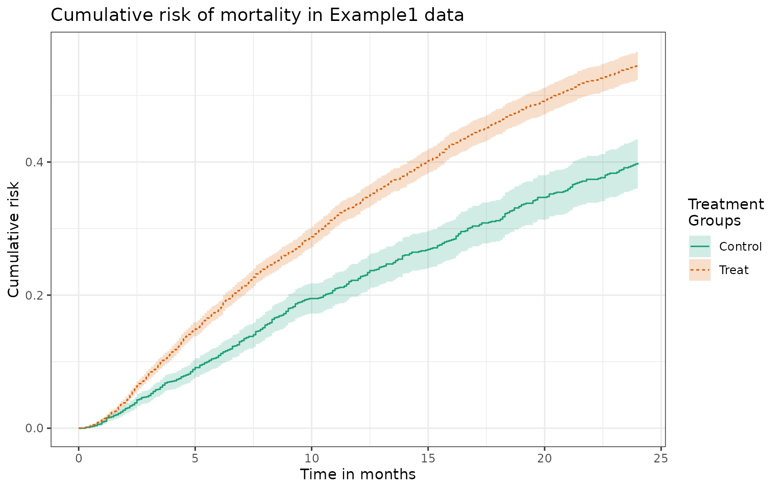
When passing the same ipw object into
plot_phr, we get a tibble containing the
cumulative risk estimates along the time sequence defined in the object
for both treatment groups.
fit1_plot_df <- plot_phr(fit1_treat)
head(fit1_plot_df)
#> # A tibble: 6 × 7
#>    time estimate       lcl     ucl group_label grp1                       grp2
#>   <dbl>    <dbl>     <dbl>   <dbl> <fct>       <fct>                      <fct>
#> 1   0    0       0         0       Control     Unadjusted cumulative risk NA
#> 2   0.1  0       0         0       Control     Unadjusted cumulative risk NA
#> 3   0.2  0       0         0       Control     Unadjusted cumulative risk NA
#> 4   0.3  0.00147 0.0000295 0.00290 Control     Unadjusted cumulative risk NA
#> 5   0.4  0.00147 0.0000295 0.00290 Control     Unadjusted cumulative risk NA
#> 6   0.5  0.00229 0.000455  0.00412 Control     Unadjusted cumulative risk NA
When plotting in causalRisk it is common to include
multiple objects and display cumulative risk or risk difference curves
using panels.
models2 = specify_models(identify_treatment(Statin, formula = ~DxRisk ),
                         identify_censoring(EndofEnrollment,
                                            formula = ~DxRisk),
                         identify_outcome(Death))

fit2 = estimate_ipwrisk(example1, models2,
                        times = seq(0,24,0.1),
                        labels = c("IPTCW main analysis"))

adj = fit2 %>%
  update_treatment(new_name = StatinPotency) %>%
  update_label("Adjusted") %>% re_estimate()

unadj = adj %>%
  update_treatment(new_formula = ~1) %>%
  update_label("Unadjusted") %>% re_estimate()

not_frail = adj %>% subgroup(Frailty > 0) %>%
  update_label("Not Frail") %>% re_estimate()

frail = adj %>% subgroup(Frailty <= 0) %>%
  update_label("Frail") %>% re_estimate()

high_risk = adj %>% subgroup(DxRisk <= 0) %>%
  update_label("High Risk") %>% re_estimate()

low_risk = adj %>% subgroup(DxRisk > 0) %>%
  update_label("Low Risk") %>% re_estimate()

plot(unadj, adj, not_frail, frail, low_risk, high_risk, effect_measure_type = "RD", scales = "fixed", ncol = 2) +
  ylab("Cumulative Risk Difference") +
xlab("Time in months") 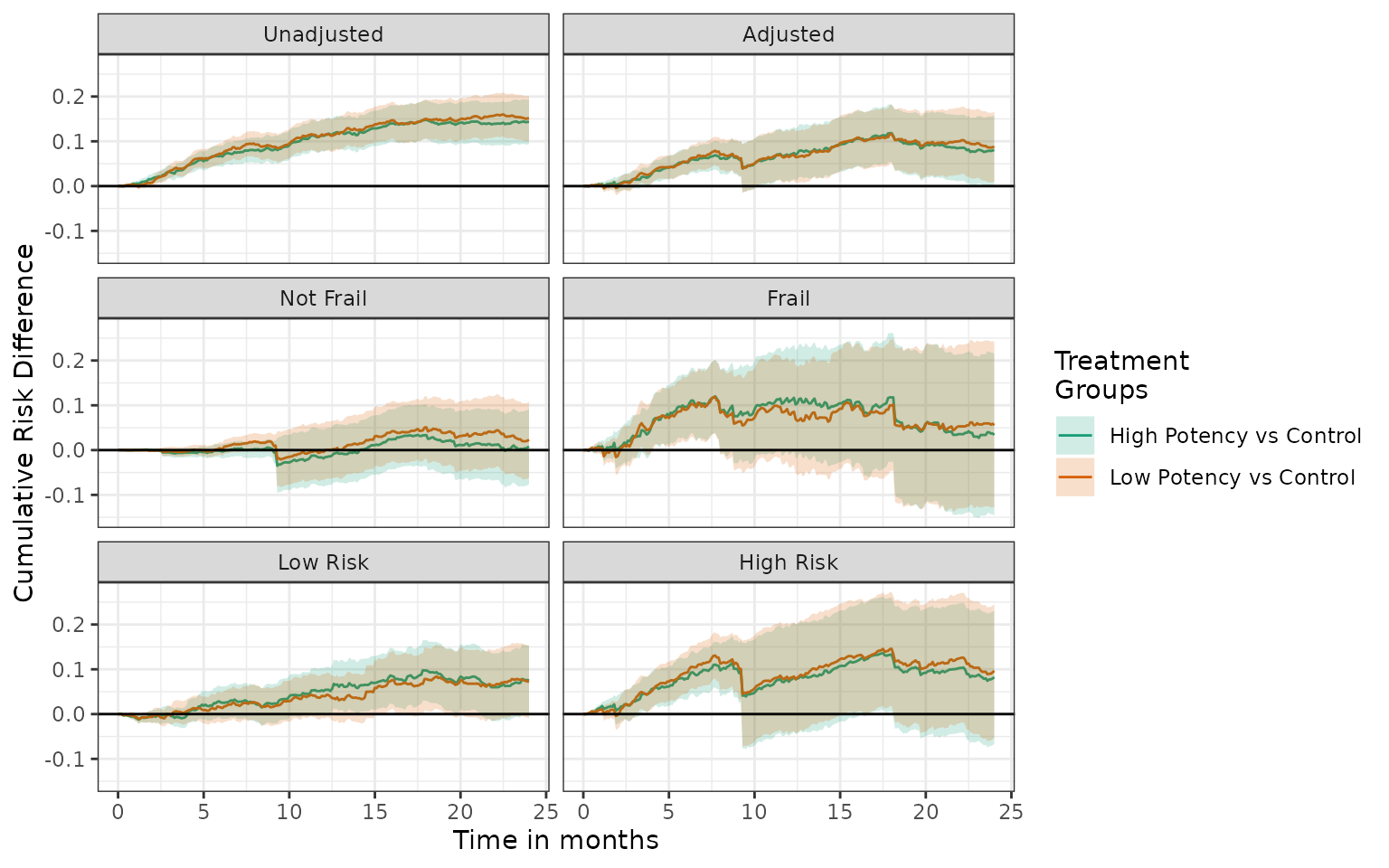
The corresponding plot_phr example produces a
tibble where each cell of the panel is indicated by the
grp1 column. Since panelling is not a capability within a
PHR plot, the individual cells can be viewed separately by using a
plot’s filters.
plot_panel_df <- plot_phr(unadj, adj, not_frail, frail, low_risk, high_risk, effect_measure_type = "RD")
head(plot_panel_df)
#> # A tibble: 6 × 7
#>    time  estimate       lcl     ucl group_label grp1       grp2
#>   <dbl>     <dbl>     <dbl>   <dbl> <fct>       <fct>      <fct>
#> 1   0    0         0        0       Low Potency Unadjusted NA
#> 2   0.1  0         0        0       Low Potency Unadjusted NA
#> 3   0.2  0         0        0       Low Potency Unadjusted NA
#> 4   0.3 -0.000490 -0.00230  0.00132 Low Potency Unadjusted NA
#> 5   0.4  0.00150  -0.000913 0.00392 Low Potency Unadjusted NA
#> 6   0.5  0.00203  -0.000950 0.00501 Low Potency Unadjusted NA
Use nswpr::import_report_data_df to upload this
tibble to studio.novisci.com. Depending on the
number of objects and treatment groups included in the
plot_phr call, the subgroups argument will
need to be specified. For example when uploading
plot_panel_df, subgroups will need to be:
c("group_label","grp1"), whereas fit1_plot_df
only requires the subgroup associated with the treatment group
(group_label). The “group_label” subgroup allows for
in-plot stratification by group while “grp1” allows for filtering to the
cell within a panel. Example
Plots
make_phr_table1
The function make_table1 can be used to tabulate summary
statistics of specified covariates by treatment group.
make_table1(example1, Statin, DxRisk, Frailty, Sex)| Characteristic1 | Control n=3201 |
Treat n=6799 |
|---|---|---|
| DxRisk, Mean (SD) | 0.74 (0.85) | -0.35 (0.88) |
| Frailty, Mean (SD) | 0.01 (1.02) | 0.02 (1.00) |
| Sex | ||
| Female | 1581 49.39 | 3287 48.35 |
| Male | 1620 50.61 | 3512 51.65 |
| 1 All values are N (%) unless otherwise specified | ||
make_phr_table1 returns a tibble with the
corresponding values and additionally assigns a cell_format
based on what each row represents (overall counts, continuous, or
categorical variables). By having multiple cell_formats
users have flexibility in how they choose to display results using
primary and secondary statistics.
make_phr_table1(example1, Statin, DxRisk, Frailty, Sex)
#> Warning in sprintf(paste0("%.", round, "f"), round(num.sum$sd, round), round):
#> one argument not used by format '%.2f'

#> Warning in sprintf(paste0("%.", round, "f"), round(num.sum$sd, round), round):
#> one argument not used by format '%.2f'

#> Warning in sprintf(paste0("%.", round, "f"), round(num.sum$sd, round), round):
#> one argument not used by format '%.2f'

#> Warning in sprintf(paste0("%.", round, "f"), round(num.sum$sd, round), round):
#> one argument not used by format '%.2f'
#>                   row  column stat1  stat2 section    n cell_format
#> 1             Overall Control  <NA>   <NA>         3201     Overall
#> 2             Overall   Treat  <NA>   <NA>         6799     Overall
#> 3   DxRisk, Mean (SD) Control  0.74 (0.85)           NA     format2
#> 4   DxRisk, Mean (SD)   Treat -0.35 (0.88)           NA     format2
#> 5  Frailty, Mean (SD) Control  0.01 (1.02)           NA     format2
#> 6  Frailty, Mean (SD)   Treat  0.02 (1.00)           NA     format2
#> 7              Female Control  1581  49.39     Sex   NA     format1
#> 8              Female   Treat  3287  48.35     Sex   NA     format1
#> 9                Male Control  1620  50.61     Sex   NA     format1
#> 10               Male   Treat  3512  51.65     Sex   NA     format1
make_phr_table2
The standard Table 2’s from cumrisk or cumcount objects consist of one row for each treatment group in each supplied object. The table contains N, person-years of follow-up, number of events, either a cumultive risk or cumulative count (at a specified time point) and a (1-alpha) confidence interval.
make_table2(fit2, risk_time = 24)
make_phr_table2(fit2, risk_time = 24)
#> # A tibble: 14 × 6
#>    row     column      value              lcl               ucl      cell_format
#>    <chr>   <chr>       <chr>              <chr>             <chr>    <chr>
#>  1 Control crisk       0.440783294965121  0.373579331704194 0.50798… CI
#>  2 Control criskfunc   NA                 NA                NA       CI
#>  3 Control events      470                NA                NA       Default
#>  4 Control n           3201               NA                NA       Default
#>  5 Control person_time 22875.1444186661   NA                NA       Default
#>  6 Control rate        0.0205463183706277 NA                NA       Default
#>  7 Control time        24                 NA                NA       Default
#>  8 Treat   crisk       0.524691612443825  0.500392662700333 0.54899… CI
#>  9 Treat   criskfunc   0.0839083174787044 0.011213760989646 0.15660… CI
#> 10 Treat   events      2099               NA                NA       Default
#> 11 Treat   n           6799               NA                NA       Default
#> 12 Treat   person_time 63932.5981510698   NA                NA       Default
#> 13 Treat   rate        0.032831451570921  NA                NA       Default
#> 14 Treat   time        24                 NA                NA       Default
make_phr_wt_summary_table
wt_summary is a function that creates a table summarizing statistics about treatment weights.
extreme_weights_phr
extreme_weights is a function that creates a table summarizing
statistics about treatment weights. When including multiple object in
the function call, subgroups = 'analysis' must be included
in the nswpr::import_report_data_df upload.
hist_phr
hist_phr is a function that takes as an argument a list of ipw
objects, or the objects provided as independent arguments. Both weighted
and unweighted estimates can be produced. The panelling style of
causalRisk::hist.ipw is captured with the
subgroup function of
nswpr::import_report_data_df
forest_plot_phr
forest_plot_phr is a function that takes as an argument a list of cumrisk objects, or the objects provided as independent arguments, each representing a set of cumulative incidence functions. The function returns a tibble containing the risk differences.
forest_plot(fit1,fit1_treat, risk_time = 24)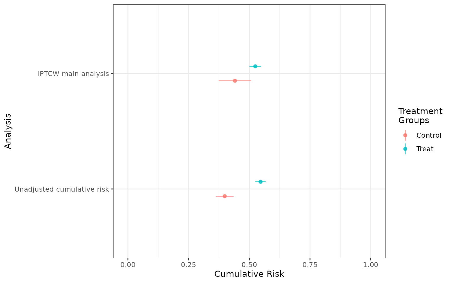
forest_plot_phr(fit1,fit1_treat, risk_time = 24)
#> # A tibble: 4 × 6
#>   analysis                   group    risk ci_lo ci_hi risk_time
#>   <fct>                      <fct>   <dbl> <dbl> <dbl>     <dbl>
#> 1 IPTCW main analysis        Control 0.441 0.374 0.508        24
#> 2 IPTCW main analysis        Treat   0.525 0.500 0.549        24
#> 3 Unadjusted cumulative risk Control 0.399 0.362 0.436        24
#> 4 Unadjusted cumulative risk Treat   0.546 0.525 0.567        24
When uploading to the platform, chart_types = "forest"
is required. Additionally, forest plots require manual configuration on
the platform at this time. Example
Forest Plot