Table Data Format
Neil Harding
2026-07-20
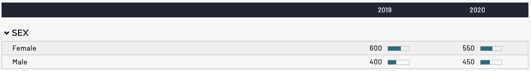
table_data_format.RmdTable data on the platform is represented by a rectangular set of data where each row in the dataset represents one “cell” in the table. Each row defines what section, row, and column that cell should be located in. It also defines a “cell format” name which will be used by the platform to fill values into the cell. Example:
read.csv('./simple_table.csv')
#>   section    row column   n percent cell_format
#> 1     Sex Female   2019 600    0.60   n_percent
#> 2     Sex   Male   2019 400    0.40   n_percent
#> 3     Sex Female   2020 550    0.55   n_percent
#> 4 Sex Male 2020 450 0.45 n_percentThe above table dataset can be imported into the platform and configured to display like this:
Cells, Values and Cell Formats
A cell in the table can contain multiple values and each value may even be displayed as a mini visualization within the table cell. An example of a cell with a simple number value and a mini bar chart representing the percentage is highlighted here:
In the simple table example at the top of the page there are columns
in the dataset named n and percent - those
contain the values that will be displayed in the cell. The
cell_format column is used by the platform’s report editor
to configure how that cell should be formatted. These
cell_format names can be anything you want - they just need
to be unique to each of the different ways cells will be formatted in
your table. In the example above I used “n_percent” because the cell is
going to display the values from the n and
percent columns.
Cells can be formatted differently within the same table. For example, you may display n in one row, but a mean and standard deviation in another row of the table:
read.csv('./different_cell_formats.csv')
#>         row column   n mean sd cell_format
#> 1 Mean (SD) Female  NA   12 15     mean_sd
#> 2 Mean (SD)   Male  NA    5 10     mean_sd
#> 3     Total Female 600   NA NA           n
#> 4     Total   Male 400   NA NA           n
Sections vs. Standalone Rows
Sections are a way to group rows together within a table. As you can see from the previous example, sections are optional. If there is no section column in the dataset, the rows will be displayed without a section title. You can mix sections with “standalone” rows within a single table. An example is an “Overall” row. In the dataset you include a section column, but specify an empty string (““) as the section value for the standalone rows. Example:
read.csv('./standalone_row.csv')
#>   section     row column    n percent cell_format
#> 1         Overall   2019 1000      NA           n
#> 2         Overall   2020 1000      NA           n
#> 3     Sex  Female   2019  600    0.60   n_percent
#> 4     Sex    Male   2019  400    0.40   n_percent
#> 5     Sex  Female   2020  550    0.55   n_percent
#> 6     Sex    Male   2020  450    0.45   n_percent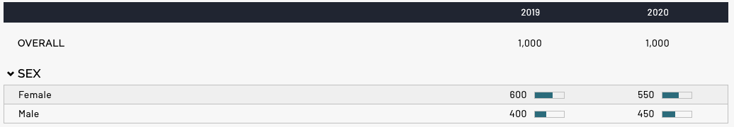
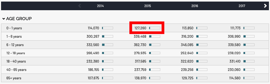
Filtering Tables
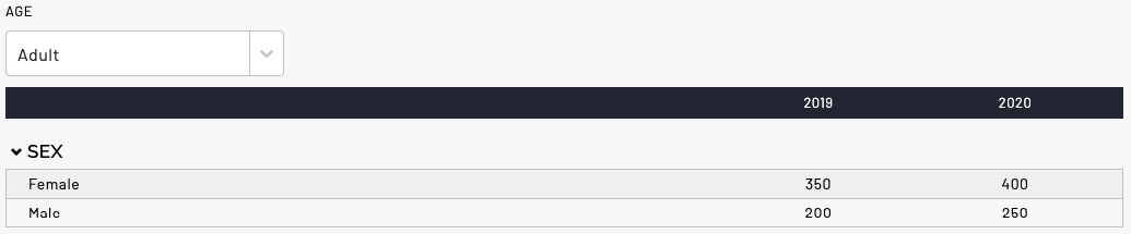
The platform supports filter dropdowns above tables - this allows the user to change the data in the table by selecting a different value in the dropdown. For example, if I want to display the data for each sex in rows, but I want a dropdown to switch between adult values and child values.
read.csv('./filterable_table.csv')
#>     age section    row column   n cell_format
#> 1 adult     Sex Female   2019 350           n
#> 2 adult     Sex   Male   2019 200           n
#> 3 adult     Sex Female   2020 400           n
#> 4 adult     Sex   Male   2020 250           n
#> 5 child     Sex Female   2019 250           n
#> 6 child     Sex   Male   2019 200           n
#> 7 child     Sex Female   2020 150           n
#> 8 child Sex Male 2020 200 nIf I select “Adult” in the dropdown, I would see this:
And if I select “Child” in the dropdown, I would see this:

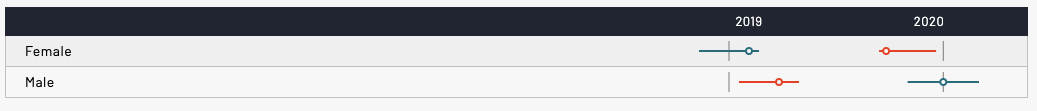
Forest Plot Table
One special cell format is the “confidence plot”. This will plot a value along with a lower and upper confidence value. When put together into a full table it becomes a multi-column forest plot. The data set to support this looks the same as the above examples. The only difference is you will need 3 value columns representing the estimate and the upper & lower confidence values. Example:
read.csv('./forest_table.csv')
#>      row column estimate lower upper cell_format
#> 1 Female   2019      1.2   0.7   1.3  confidence
#> 2   Male   2019      1.5   1.1   1.7  confidence
#> 3 Female   2020      0.2   0.1   0.9  confidence
#> 4   Male   2020      1.0   0.5   1.5  confidence